Solow Model and Regression Analyses
Another popular approach of taking the Solow model to data is to use growth regressions, which involve estimating regression models with country growth rates on the left-hand side.
These growth regressions have been used extensively following the work by Barro (1991). To see how these regressions are motivated and what their shortcomings are, let us return to the basic Solow model with constant population growth and labor-augmenting technological change in continuous time. Recall that, in this model, the equilibrium is described by the following equations:(3.6)
and
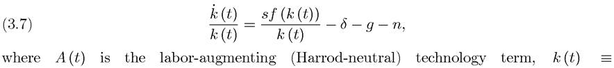
K (t) / (A (t) L (t)) is the effective capital labor ratio and f (∙) is the per capita production function. Equation (3.7) follows from the constant technological progress and constant population growth assumptions, Now differentiating (3.6)
with respect to time and dividing both sides by y (t),
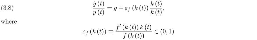
is the elasticity of the f (∙) function. The fact that it is between 0 and 1 follows from Assumption 1. For example, with the Cobb-Douglas technology from Example 2.1 in the previous chapter, εf (k (t)) = α, that is, it is a constant independent of k (t) (see Example 3.1 below). However, generally, this elasticity is a function of k (t).
Now let us consider a first-order Taylor expansion of (3.7) with respect to log k (t) around the steady-state value k* (and recall that This expansion implies
that for k (t) in the neighborhood of k*, we have
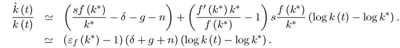
The use of the symbol “'” here is to emphasize that this is an approximation, ignoring second-order terms.
In particular, the first line follows simply by differentiating k (t) /k (t) with respect to log k (t) and evaluating the derivatives at k* (and ignoring second-order terms). The second line uses the fact that the first term in the first line is equal to zero by definition of the steady-state value k* (recall that from eq. (2.48) in the previous chapter,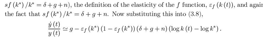 ι
ι
Let us define y* (t) ? A (t) f (k*) as the “steady-state level of output per capita,” that is, the level of per capita output that would apply if the effective capital-labor ratio were at its steady-state value and technology were at its time t level. A first-order Taylor expansion of log y (t) with respect to log k (t) around log k* (t) then gives

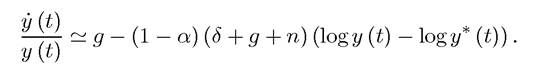
Combining this with the previous equation yields the following “convergence equation”:

Equation (3.9) makes it clear that, in the Solow model, there are two sources of growth in output per capita: the first is g, the rate of technological progress, and the second is “convergence”. This latter is a consequence of the impact of the gap between the current level of output per capita and the steady-state level of output per capita on the rate of capital accumulation (recall that Intuitively, the further is a country below
its steady-state capital-labor ratio, the more capital it will accumulate and the faster it will grow. Put differently, the lower is y (t) relative to y* (t), and thus the lower is k (t) relative to k*, the greater is the average product of capital f (k*) /k*, and this leads to faster growth in the effective capital-labor ratio. This pattern is already visible in Figure 2.7 in the previous chapter.
Another noteworthy feature is that the speed of convergence in eq. (3.9), measured by the term multiplying the gap between log y (t) and log y* (t), depends on
δ + g + n, and on the elasticity of the production function, Both of these capture intuitive effects. As discussed in the previous chapter, the term δ + g + n determines the rate at which the effective capital-labor ratio needs to be replenished. The higher is this rate of replenishment, the larger is the amount of investment in the economy (recall Figure 2.7 in the previous chapter) and thus there is room for faster adjustment. On the other hand, when εf (k*) is high, we are close to a linear—AK—production function, and as demonstrated in the previous chapter, in this case convergence should be slow. In the extreme case where εf (k*) is equal to 1, the economy takes the AK form and there is no convergence.
EXAMPLE 3.1. (Cobb-Douglas Production Function and Convergence) Consider briefly the Cobb-Douglas production function from Example 2.1 in the previous chapter, where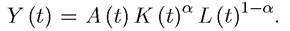 This implies that
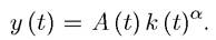 Consequently, as
noted above, εf (k (t)) = α. Therefore, (3.9) becomes
This equation also enables us to “calibrate” the speed of convergence in practice—meaning to obtain a back-of-the-envelope estimate of the speed of convergence by using plausible values of parameters. Let us focus on advanced economies. In that case, plausible values for these parameters might be g ' 0.02 for approximately 2% per year output per capita growth, n ' 0.01 for approximately 1% population growth and δ ' 0.05 for about 5% per year depreciation.
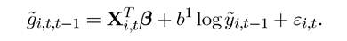
Recall also from the previous chapter that the share of capital in national income is about 1/3, so with the Cobb-Douglas production function we should have α ' 1/3. Consequently, we may expect the convergence coefficient in front of log y (t) — log y* (t) to be around 0.054 (' 0.67 ? 0.08). This is a very rapid rate of convergence and would imply that the income gap between two similar countries that have the same technology, the same depreciation rate and the same rate of population growth should narrow rather quickly. For example, it can be computed that with these numbers, the gap of income between two similar countries should be halved in little more than 10 years (see Exercise 3.4). This is clearly at odds with the patterns we saw in Chapter 1.Next using a discrete-time approximation, eq. (3.9) yields the regression equation:  where gi,ty-i is the growth rate of country i between dates t — 1 and t, log yit-ι is the “initial” (time t — 1) log output per capita of this country, and ε^t is a stochastic term capturing all omitted influences. Regressions on this form have been estimated by, among others, Baumol (1986), Barro (1991) and Barro and Sala-i-Martin (1992). If such an equation is estimated in the sample of core OECD countries, b1 is indeed estimated to be negative; countries like Greece, Spain and Portugal that were relatively poor at the end of World War II have grown faster than the rest as shown in Figure 1.14 in Chapter 1.
Yet, Figure 1.13 in Chapter 1 shows, when we look at the whole world, there is no evidence for a negative b1. Instead, this figure makes it clear that, if anything, b1 would be positive. In other words, there is no evidence of world-wide convergence.
Barro and Sala-i-Martin refer to this type of convergence as “unconditional convergence,” meaning the convergence of countries regardless of differences in characteristics and policies.
However, this notion of unconditional convergence may be too demanding. It requires that there should be a tendency for the income gap between any two countries to decline, regardless of the technological opportunities, investment behavior, policies and institutions of these countries. If they do differ with respect to these factors, the Solow model would not predict that they should converge in income level. Instead, each should converge to their own level of steady-state income per capita or balanced growth path. Thus in a world where countries differ according to their characteristics, a more appropriate regression equation may take the form:
where the key difference is that now the constant term, , is country specific. (In principle, the slope term, measuring the speed of convergence, b1, should also be country specific, but in empirical work, this is generally taken to bea constant, and I assume the same here to simplify the exposition). One may then model
 as a function of country characteristics.
If the true equation is (3.11), in the sense that the Solow model applies but certain determinants of economic growth differ across countries, eq. (3.10) would not be a good fit to the data. Put differently, there is no guarantee that the estimates of b1 resulting from this equation will be negative. In particular, it is natural to expect that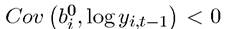
(where Cov refers to the population covariance), since economies with certain growth-reducing characteristics will have low levels of output. This implies a negative bias in the estimate of b1 in eq. (3.10), when the more appropriate equation is (3.11).
With this motivation, Barro (1991) and Barro and Sala-i-Martin (1992, 2004) favor the notion of “conditional convergence,” which means that the convergence effects emphasized by the Solow model should lead to negative estimates of b1 once is allowed to vary across countries. To implement this idea of conditional convergence empirically, they estimate models where b0 is assumed to be a function of, among other things, the male schooling rate, the female schooling rate, the fertility rate, the investment rate, the government-consumption ratio, the inflation rate, changes in terms of trades, openness and institutional variables such as rule of law and democracy. In regression form, this can be written as

where is a (column) vector including the variables mentioned above (as well as a constant), with a vector of coefficients β (recall that
 denotes the transpose of X). In other words, this specification imposes that
 in eq. (3.11) can be approximated by
 Consistent with the emphasis on conditional convergence, regressions of eq. (3.12) tend to show a negative estimate of b[III], but the magnitude of this estimate is much lower than that suggested by the computations in Example 3.1.
Regressions similar to (3.12) have not only been used to support “conditional convergence,” but also to estimate the “determinants of economic growth”. In particular, it may appear natural to presume that the estimates of the coefficient vector β will contain information about the causal effects of various variables on economic growth. For example, the fact that the schooling variables enter with positive coefficients in the estimates of regression (3.12) is interpreted as evidence that “schooling causes growth”. The simplicity of the regression equations of the form (3.12) and the fact that they create an attractive bridge between theory and data have made them very popular over the past two decades.
Nevertheless, there are several problematic features with regressions of this form. These include:
1. Most, if not all, of the variables in as well as logyit-1, are econometrically endogenous in the sense that they are jointly determined with the rate of economic growth between dates t — 1 and t. For example, the same factors that make a country relatively poor in 1950, thus reducing logyit-1, should also affect its growth rate after 1950. Or the same factors that make a country invest little in physical and human capital could have a direct effect on its growth rate (through other channels such as its technology or the efficiency with which the factors of production are being utilized). This creates an obvious source of bias (and lack of econometric consistency) in the regression estimates of the coefficients. This bias makes it unlikely that the effects captured in the coefficient vector β correspond to causal effects of these characteristics on the growth potential of economies. One may argue that the convergence coefficient b1 is of interest, even if it does not have a “causal interpretation”. This argument is not entirely compelling, either. A basic result in econometrics is that if
is econometrically endogenous, so that the parameter vector β is estimated inconsistently, the estimate of the parameter b1 will also be inconsistent unless is independent from logyig-i.1 This makes the estimates of the convergence coefficient, b1, difficult to interpret.
2. Even if thrn were econometrically exogenous, a negative coefficient estimate for b1
could be caused by other econometric problems, such as measurement error or other transitory shocks to yiy. For example, because national accounts data are measured with error, data on log yig will naturally contain measurement error. Suppose, for example, that we only observe estimates of output per capita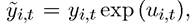 where y^t is the true output per capita
and Uit is a random and serially uncorrelated error term. When the variable log yit is used in the regression, the error term Uijt-1 appears both on the left-hand side and the right-hand side of (3.12). In particular, note that

the measurement error Uijt-1 will be part of both the error term and the right-hand side variable log yit-ι = log yit-ι + in the regression equation
This will naturally lead a negative bias in the estimation of b1. Therefore, we can end up with a negative estimate of b1, even when there is no conditional convergence.
3. The economic interpretation of regression equations like (3.12) is not always straightforward either. Many of the regressions used in the literature include the investment rate as part of the vector (and all of them include the schooling rate). However, in the Solow model, differences in investment rates are the channel via which convergence takes place—in the sense that economies below their steady state grow faster by having higher investment rates. Therefore, according to the Solow model, conditional on the investment rate there should be no further effect of the gap between the current level of output and the steadystate level of output. The same concern applies to the interpretation of the effects of the variables in
 (such as institutions or openness), which are typically included as potential determinants of economic growth. However, many of these variables affect growth primarily by affecting the investment rate (or the schooling rate). Therefore, once we condition on the investment rate and the schooling rate, the coefficients on these variables no longer measure their impact on economic growth. Consequently, estimates of (3.12) with investment-like variables on the right-hand side are difficult to link to theory.
4. Regressions of the form (3.12) are often thought to be appealing because they model the
“process of economic growth” and may give us information about the potential determinants of economic growth (to the extent that these are included in the vector Nevertheless, there is a sense in which growth regressions are not much different than “levels regressions” — similar to those discussed in Section 3.4 below and further in Chapter 4. In particular, again noting that
 (3.12) can be rewritten as

Therefore, essentially the level of output is being regressed on so that regression of the form (3.12) will typically uncover the correlations between the variables in the vector
 and output per capita. Thus growth regressions are often informative about which economic or social processes go hand-in-hand with high levels of output. A specific example is life expectancy. When life expectancy is included in the vector
 in a growth regression, it is often highly significant. But this simply reflects the high correlation between income per capita and life expectancy (recall Figure 1.6 in Chapter 1). It does not imply that life expectancy has a causal effect on economic growth, and more likely, it reflects the joint determination of life expectancy and income per capita and the impact of prosperity on life expectancy.
5. Finally, the motivating equation for the growth regression, (3.9), is derived for a closed Solow economy. When we look at cross-country income differences or growth experiences, the use of this equation imposes the assumption that “each country is an island”. In other words, the world is being interpreted as a collection of non-interacting closed economies. In
practice, countries trade goods, exchange ideas and borrow and lend in international financial markets. This implies that the behavior of different countries will not be given by eq. (3.9), but by a system of equations characterizing the joint world equilibrium. Even though a world equilibrium is typically a better way of representing differences in income per capita and their evolution, in the first part of the book I follow the usual approach of treating “each country as an island,” which is simpler and thus a useful starting point to develop the main ideas. I return to models of world equilibrium in Chapters 18 and 19.
This discussion suggests that growth regressions need to be used with caution and ought to be supplemented with other methods of mapping the basic Solow model to data. What other methods will be useful in empirical analyses of economic growth? A number of answers emerge from our discussion above. To start with, for many of the central questions of economic growth, regressions that control for fixed country characteristics might be equally useful as, or more useful than, cross-sectional growth regressions. For example, a more natural regression framework for investigating the economic (or statistical) relationship between the variables in the vector and economic growth might be

where δj,s denote a full set of country fixed effects and μt's denote a full set of year effects. This regression framework differs from the growth regressions in a number of respects. First, the regression equation is specified in levels rather than with the growth rate on the lefthand side. But this is mainly a rearrangement of (3.13). More importantly, by including the country fixed effects, this regression equation takes out fixed country characteristics that might be simultaneously affecting economic growth (or the level of income per capita) and the right-hand side variables of interest. For instance, in terms of the example discussed in (4) above, if life expectancy and income per capita are correlated because of some omitted factors, the country fixed effects, the δj,s, will remove the influence of these factors. Therefore, panel data regressions as in (3.13) may be more informative about the relationship between a range of factors and income per capita. Nevertheless, it is important to emphasize that including country fixed effects is not a panacea against all omitted variable biases and econometric endogeneity problems. Simultaneity bias often results from time-varying influences, which cannot be removed by including fixed effects. Moreover, to the extent that some of the variables in the vector are slowly-varying themselves, the inclusion of country fixed effects will make it difficult to uncover the statistical relationship between these variables and income per capita, and may increase potential biases due to measurement error in the right-hand side variables.
This discussion highlights that econometric models similar to (3.13) are often useful and a good complement to (or substitute for) growth regressions. But they are not a good substitute for specifying the structural economic relationships fully and estimating the causal relationships of interest. The next chapter shows how some progress can be made in this regard by looking at the historical determinants of long-run economic growth and using 92
specific historical episodes to generate potential sources of exogenous variation in the variables of interest that can allow us to develop an instrumental-variables strategy.
In the remainder of this chapter, I discuss how the structure of the Solow model can be further exploited to look at the data. Before doing this, I present an augmented version of the Solow model incorporating human capital, which is useful in these empirical exercises.
3.3.