The Solow Model with Human Capital

Human capital is a term we use to represent the stock of skills, education, competencies and other productivity-enhancing characteristics embedded in labor. Put differently, human capital represents the efficiency units of labor embedded in raw labor hours.

The term “human capital” originates from the observation that individuals will invest in their skills, competencies and earning capacities in the same way as firms invest in their physical capital—to increase their productivity. The seminal work by Ted Schultz, Jacob Mincer and Gary Becker brought the notion of human capital to the forefront of economics. For now, all we need to know is that labor hours supplied by different individuals do not contain the same efficiency units; a highly trained carpenter can produce a chair in a few hours, while an amateur would spend many more hours to perform the same task. Economists capture this notion by thinking that the trained carpenter has more efficiency units of labor embedded in the labor hours he supplies, or alternatively he has more human capital. The theory of human capital is very rich and some of the important notions will be discussed in Chapter 10. For now, our objective is more modest, to investigate how including human capital makes the Solow model a better fit to the data. The inclusion of human capital will enable us to embed all three of the main proximate sources of income differences; physical capital, human capital and technology.

For the purposes of this section, let us focus on the continuous-time economy and suppose that the aggregate production function of the economy is given by a variant of eq. (2.1): (3.14) Y = F (K, H, AL), where H denotes “human capital”. Notice that this production function is somewhat unusual, since it separates human capital H from labor L as potential factors of production. I start with this form because it is used commonly in the growth literature.

Let us also modify Assumptions 1 and 2 as follows

Assumption 1⁰: The production functionin (3.14) is twice differen-

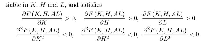
Moreover, F exhibits constant returns to scale in its three arguments.

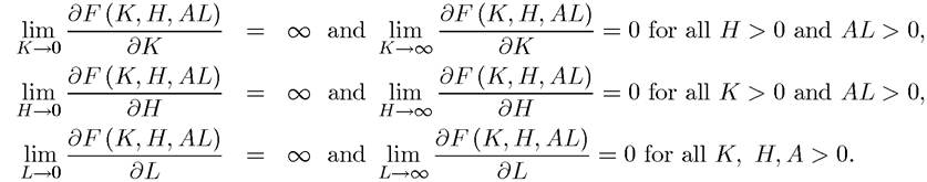
Assumption 20: F satisfies the Inada conditions

Let us assume that investments in human capital take a similar form to investments in

physical capital; households save a fraction ⅝ of their income to invest in physical capital

and a fraction.⅛ to invest in human capital. Human capital also depreciates in the same

way as physical capital, and we denote the depreciation rates of physical and human capital by δk and δh, respectively.

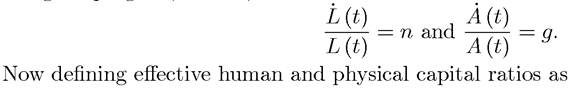
There is again constant population growth and a constant rate of labor-augmenting tech-

nological progress, that is,

and using the constant returns to scale feature in Assumption 10, output per effective unit of

labor can be written as

With the same steps as in Chapter 2, the law of motion of k (t) and h (t) can then be obtained

as:

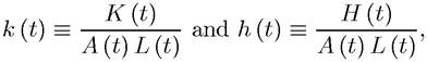
A steady-state equilibrium is now defined not only in terms of effective capital-labor ratio, but effective human and physical capital ratios, (k*,h*), which satisfy the following two equations:

and

As in the basic Solow model, the focus is on steady-state equilibria with k* > 0 and h* > 0 (if f (0, 0) = 0, then there exists a trivial steady state with k = h = 0, which I ignore for the same reasons as in the previous chapter).

Let us first prove that this steady-state equilibrium is unique.

Figure 3.1. Steady-state equilibrium in the Solow model with human capital.

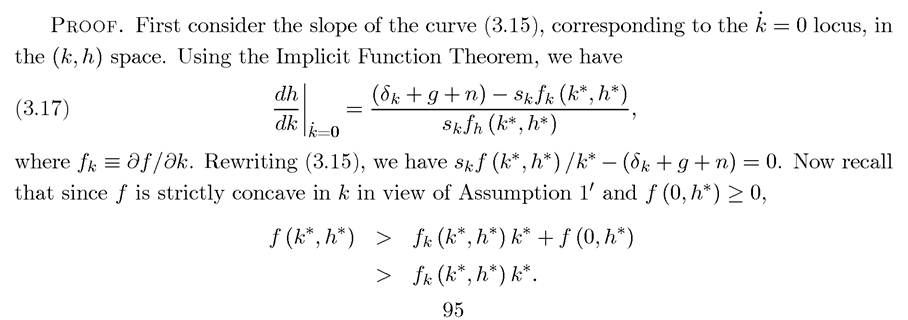
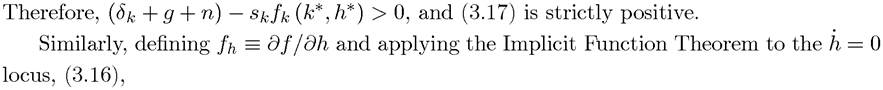
PROPOSITION 3.1. Suppose Assumptions 1' and 20 are satisfied. Then, in the augmented Solow model with human capital, there exists a unique steady-state equilibrium (k*,h*).

With the same argument as that used for (3.17), this expression is also strictly positive.

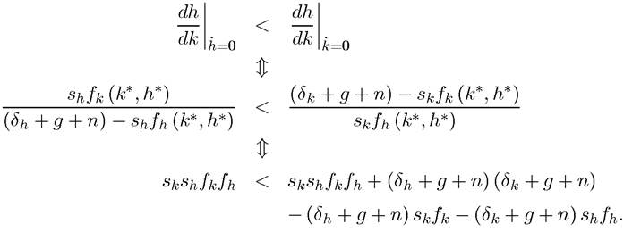
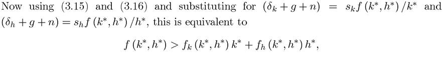
Next, we prove that (3.17) is steeper than (3.18) whenever (3.15) and (3.16) hold, so that can it most be one intersection. First, observe that

This proposition shows that a unique steady state exists when the Solow model is aug­mented with human capital. The comparative statics are similar to the basic Solow model (see Exercise 3.7). Most importantly, both greater s⅛ and greater.⅛ will translate into higher normalized output per capita, y*.

Now turning to cross-country behavior, consider a set of countries experiencing the same rate of labor-augmenting technological progress, g. Then, those with greater propensity to invest in physical and human capital will bthise relatively richer. This is the type of prediction that can be investigated empirically to see whether the augmented Solow model (with similar technological possibilities across countries) provides us with a useful way of looking at cross-country income differences.

Before doing this, however, let us verify that the unique steady state is globally stable. The next proposition shows that this is the case.

PROPOSITION 3.2. Suppose Assumptions 1' and 20 are satisfied. Then, the unique steady­state equilibrium of the augmented Solow model with human capital, (k*,h*), is globally stable in the sense that starting with any k (0) > 0 and h (0),

Proof. See Exercise 3.6. ?

Figure 3.2 gives the intuition for this result, by showing the law of motion of k and h depending on whether the economy is above or below the two curves representing the loci for k = 0 and h = 0, respectively, (3.15) and (3.16). When we are to the right of the (3.15) curve, there is too much physical capital relative to the amount of labor and human capital, and consequently, ę < 0. When we are to its left, we are in the converse situation and ę > 0. Similarly, when we are above the (3.16) curve, there is too little human capital relative to the amount of labor and physical capital, and thus h > 0. When we are below it, h < 0. Given these arrows, the global stability of the dynamics follows.

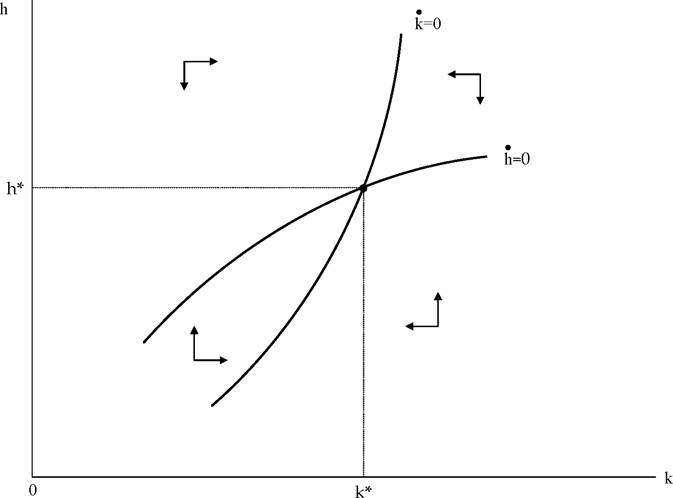
FlgURE 3.2. Dynamics of physical capital-labor and human capital-labor ra­tios in the Solow model with human capital.

ExaMPlE 3.2. (Augmented Solow Model with Cobb-Douglas Production Func­tions) Let us now work through a special case of the above model with Cobb-Douglas production function.

(3.19)

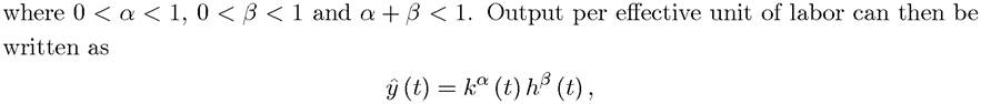
which shows that a higher saving rate in physical capital not only increases k*, but also h*. The same applies for a higher saving rate in human capital. This reflects the facts that the higher saving rate in physical capital, by increasing, k*, raises overall output and thus the amount invested in schooling (since ⅜ is constant). Given (3.20), output per effective unit of labor in steady state is obtained as

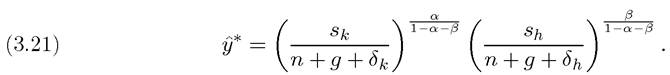
This expression shows that the relative contributions of the saving rates for physical and human capital on (normalized) output per capita depends on the shares of physical and human capital—the larger is α, the more important is ⅜ and the larger is β, the more important is ⅜.

3.4.