Solow Model and Cross-Country Income Differences: Regression Analyses

3.4.1. A World of Augmented Solow Economies. An important paper by Mankiw, Romer and Weil (1992) used regression analysis to take the augmented Solow model, with human capital, to data.

Mankiw, Romer and Weil, like many other authors, start with the assumption mentioned above, that “each country is an island”; in other words, they assume that countries do not interact (perhaps except for sharing some common technology growth, see below). This assumption enables us to analyze the behavior of each economy as a self-standing Solow model. Even though “each country is an island” is an unattractive assumption, it is a useful starting point both because of its simplicity and because this is where much of the literature started from (and in fact, it is still where much of the literature stands).

Following Example 3.2, let us assume that country j = 1,...,N has the aggregate pro­duction function: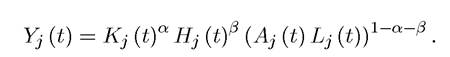

This production function nests the basic Solow model without human capital when α = 0. First, assume that countries differ in terms of istheir saving rates, s⅛ j and Sh j, population

Since our main interest here is cross-country income differences, rather than studying the dynamics of a particular country over time, let us focus on a world in which each country is in steady state (thus ignoring convergence dynamics, which was the focus in the previous section). To the extent that countries are not too far from their steady state, there will be little loss of insight from this assumption, though naturally this approach will not be satisfactory when we think of countries experiencing very large growth spurts or growth collapses, as in some of the examples discussed in Chapter 1.

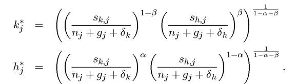
Given the steady-state assumption, equivalents of eq.’s (3.20) apply here and imply that the steady state physical and human capital to effective labor ratios of country are given by:

Consequently, using (3.21), the “steady-state” income per capita of country j can be written

as

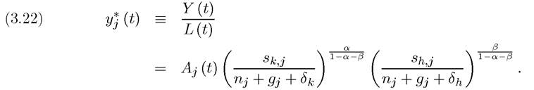
Here yj (t) stands for output per capita of country j along the balanced growth path. An immediate implication of this equation is that if g_j∙’s are not equal across countries, income per capita will diverge, since the terms in front, thewill be growing at different rates for different countries. As discussed in Chapter 1, there is some evidence for this type of divergent behavior, but the world (per capita) income distribution can also be approximated by a relatively stable distribution. Recall that this is an area of current research and there is an active debate on whether the world economy in the postwar era should be modeled as having an expanding or a stable distribution of income per capita. The former would be consistent with a specification in which thediffer across countries, while the latter would

require all countries to have the same rate of technological progress, g (recall the discussion in Chapter 1).

Since technological progress is taken as exogenous in the Solow model, it is, in many ways, more appropriate for the Solow model to assume a common rate of technical progress. Motivated by this, Mankiw, Romer and Weil make the following assumption:

99

Common technology advances assumption: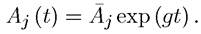

That is, countries differ according to their technology level, in particular, according to their initial level of technology, Aj, but they share the same common technology growth rate, g.

Now using this assumption together with (3.22) and taking logs, we obtain the following convenient log-linear equation for the balanced growth path of income for country j = 1.....N: This is a simple and attractive equation, and can be estimated easily with cross-country data. Estimates for Skj, Sh j and nj can be computed from the available data, and combined with values for the constants δk, δh and g, these can be used to construct measures of the two key right-hand side variables. Given these measures, eq. (3.23) can be estimated by ordinary least squares (by regressing income per capita on these measures) to uncover the values of α and β.

Mankiw, Romer and Weil takeas approximate depreciation

rates for physical and human capital and as the growth rate for the world economy. These numbers are somewhat arbitrary, but their exact values are not important for the estimation. The literature typically approximates s∣._j with average investment rates (investments/GDP). Investment rates, average population growth rates nj, and log output per capita are from the Summers-Heston dataset discussed in Chapter 1. In addition, they use estimates of the fraction of the school-age population that is enrolled in secondary school as a measure of the investment rate in human capital, Shj. I return to a discussion of this variable below.

However, even with all of these assumptions, eq. (3.23) can still not be estimated con­sistently. This is because the lnterm is unobserved (at least to the econometrician) and thus will be captured by the error term. Most reasonable models of economic growth would suggest that technological differences, the ln, should be correlated with investment rates

in physical and human capital.

Orthogonal technology assumption:with εj orthogonal to all other

variables.

Under the orthogonal technology assumption, lnwhich is part of the error term, is orthogonal to the key right-hand side variables and eq. (3.23) can be estimated consistently.

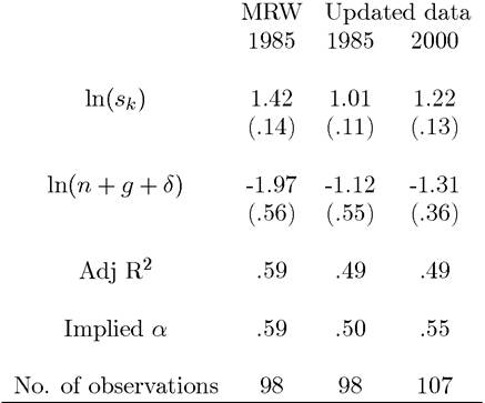
3.4.2. Mankiw, Romer and Weil Estimation Results. Mankiw, Romer and Weil first estimate eq. (3.23) without the human capital term (that is, imposing α = O) for the cross-sectional sample of non-oil producing countries. In particular, their estimating equation in this case is:

This equation is obtained from (3.23) by setting β = 0 and specializing it to a single cross section. In addition, the terms ln (s⅛ j) and ln (nj + g + δ∕,∙) are separated to test the restric­tion that their coefficients should be equal in absolute value and of opposite signs. Finally, this equation also includes εj as an error term, capturing all omitted factors and influences on income per capita.

Their results from this estimation exercise are replicated in columns 1 of Table 3.1 using the original Mankiw, Romer and Weil data (standard errors in parentheses). Their estimates suggest a coefficient of around 1.4 for α/ (1 — α), which implies that α must be around 2/3. Since α is also the share of capital in national income, it should be around 1/3. Thus, the regression estimates without human capital appear to lead to overestimates of α.

_______________ Table 3.1________________ Estimates of the Basic Solow Model

The most natural reason for the high implied values of the parameter α in Table 3.1 is thatis correlated witheither because the orthogonal technology assumption is not a good approximation to reality or because there are also human capital differences correlated withso that there is an omitted variable bias.

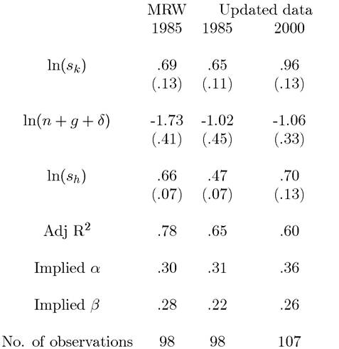
Mankiw, Romer and Weil favor the second interpretation and estimate the augmented model, in particular the equation

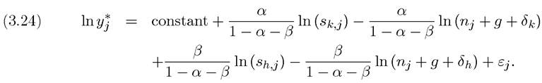
This requires a proxy for ln(⅝j). Mankiw, Romer and Weil use the fraction of the working age population that is in school. With this proxy and again under the orthogonal technology assumption, the original Mankiw, Romer and Weil estimates are given in column 1 of Table

3.2. Now the estimation is more successful. Not only is the Adjusted R² quite high (about 78%), the implied value for α is around 1/3. On the basis of this estimation result, Mankiw, Romer and Weil and others have interpreted the fit of the augmented Solow model to the data as a success: with common technology, human and physical capital investments appear to explain 78% of the cross-country income per capita differences and the implied parameter values are reasonable.

__________________ Table 3.2____________________ Estimates of the Augmented Solow Model

To the extent that these regression results are reliable, they give a big boost to the augmented Solow model. In particular, the estimate of Adjusted R² suggests that over (or close to) three quarters of income per capita differences across countries can be explained by differences in their physical and human capital investment behavior. The immediate implication is that technology (TFP) differences have a somewhat limited role, confined to at most accounting for about a quarter of the cross-country income per capita differences. If this conclusion were appropriate, it would imply that, as far as the proximate causes of prosperity are concerned, we could confine our attention to physical and human capital, and also assume that countries have access to more or less the same world technology. The implications for the modeling of economic growth are of course quite major.

The next subsection, however, will question the conclusion that technology differences are small and that physical and human capital differences are the ma jor proximate cause of income per capita differences.

3.4.3. Challenges to the Regression Analyses of Growth Models. There are two major (and related) problems with this approach.

The first relates to the assumption that technology differences across countries are or­thogonal to all other variables. While the constant technology advances assumption may be defended, the orthogonality assumption is too strong, almost untenable. When Aj varies across countries, it should also be correlated with measures ofcountries that are

more productive also invest more in physical and human capital. This is for two reasons. The first is a version of the omitted variable bias problem; technology differences are also outcomes of investment decisions. Thus societies with high levels ofwill be those that 103

have invested more in technology for various reasons; it is then natural to expect the same reasons to induce greater investment in physical and human capital as well. Second, even ignoring the omitted variable bias problem, there is a reverse causality problem; complemen­tarity between technology and physical or human capital imply that countries with high Aj will find it more beneficial to increase their stock of human and physical capital.

In terms of the regression eq. (3.24), this implies that the key right-hand side variables are correlated with the error term,Consequently, ordinary least squares regressions of eq. (3.24) will lead to upwardly biased estimates of α and β. In addition, the estimate of the R², which is a measure of how much of the cross-country variability in income per capita can be explained by physical and human capital, will also be biased upwards.

The second problem relates to the magnitudes of the estimates of α and β in eq. (3.24). The regression framework above is attractive in part because we can gauge whether the estimate of α was plausible. We should do the same for the estimate of β. However, such an exercise reveals that the coefficient on the investment rate in human capital,appears too large relative to microeconometric evidence.

Recall first that Mankiw, Romer and Weil use the fraction of the working age population enrolled in school. This variable ranges from 0.4% to over 12% in the sample of countries used for this regression. Their estimates therefore imply that, holding all other variables constant, a country with approximately 12% school enrollment should have income per capita about 9 times that of a country withMore explicitly, the predicted log difference in incomes between these two countries is

This implies that, holding all other factors constant, a country with school enrollment of over 12% should be about exp (2.24) — 1 ≈ 8.5 times richer than a country with a level of schooling investment of around 0.4.

In practice, the difference in average years of schooling between any two countries in the Mankiw-Romer-Weil sample is less than 12. Chapter 10 will show that there are good economic reasons to expect additional years of schooling to increase earnings proportionally, for example as in Mincer regressions of the form:

where Wi denotes the wage earnings of individual i, Xi is a set of demographic controls, and Si is years of schooling. The estimate of the coefficient φ is the rate of returns to education, measuring the proportional increase in earnings resulting from one more year of schooling. The microeconometrics literature suggests that eq. (3.25) provides a good approximation to the data and estimates φ to be between 0.06 and 0.10, implying that a worker with one more year of schooling earns about 6 to 10 percent more than a comparable worker with one less year of schooling. If labor markets are competitive, or at the very least, if wages are, on average, proportional to productivity, this also implies that one more year of schooling increases worker productivity by about 6 to 10 percent.

Can we deduce from this information how much richer a country with 12 more years of average schooling should be? The answer is yes, but with two caveats. First, we need to assume that the micro-level relationship as captured by (3.25) applies identically to all countries. In other words, the implicit assumption in wage regressions in general, and in eq. (3.25) in particular, is that the human capital (and the earnings capacity) of each individual is a function of his or her years of schooling. For example, ignoring other potential determinants, the wage earnings of individual i is a function of his or her schooling and can be written as 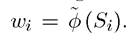The first key assumption is that this φ function is identical across countries and can be approximated by an exponential function of the form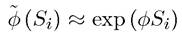so that

we obtain eq. (3.25). The reasons why this may be a reasonable assumption will be further discussed in Chapter 10.

Second, we need to assume that there are no human capital externalities —meaning that the human capital of a worker does not directly increase the productivity of other workers. There are reasons for why human capital externalities may exist and some economists believe that they are important. This evidence discussed in Chapter 10, however, suggests that human capital externalities—except those working through innovation—are unlikely to be very large. Thus it is reasonable to start without them. The key result which will enable us to go from the microeconometric wage regressions to cross-country differences is that, with constant returns to scale, perfectly competitive markets and no human capital externalities, differences in worker productivity directly translate into differences in income per capita. To see this, suppose that each firm f in country j has access to the production function

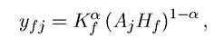
where Aj is the productivity of all the firms in the country, Kf is the capital stock and Hf denotes the efficiency units of human capital employed by firm f (thus here the production function takes the more usual form where human capital is embedded in workers rather than the form in (3.14)). Here the Cobb-Douglas production function is chosen for simplicity and does not affect the argument. Suppose also that firms in this country face a cost of capital equal to Rj. With perfectly competitive factor markets, profit maximization implies that the cost of capital must equal its marginal product,

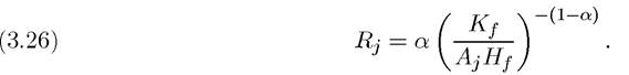
This implies that all firms ought to function at the same physical to human capital ratio, and consequently, all workers, regardless of their level of schooling, ought to work at the same physical to human capital ratio. Another direct implication of competitive labor markets is that in country j, wages per unit of human capital will be equal to

Consequently, a worker with human capital hi will receive a wage income of Wjhi. Once again, this is a more general result; with aggregate constant returns to scale production technology, wage earnings are linear in the effective human capital of the worker, so that a 105

worker with twice as much effective human capital as another should earn twice as much as this other worker (see Exercise 3.9). Next, substituting for capital from (3.26), we have total income in countrywhere Hj is the total efficiency

units of labor in country j. This equation implies that ceteris paribus (in particular, holding constant capital intensity corresponding to Rj and technology, Aj), a doubling of human capital will translate into a doubling of total income. Notice that both Aj and Rj are being kept constant here. While it may be reasonable to keep technology, A_j, constant, one may wonder whether R_j is likely change systematically in response to changes in H_j. Even though this is a possibility, such changes are likely to be small in practice. First, international capital flows will reduce the sensitivity of the rate of return to capital to domestic labor supply (see Chapter 19). Second, recall that Theorem 2.6 established the constancy of the capital-labor ratio as a requirement for a balanced growth path, and R_j will indeed be constant when the capital-labor ratio is constant (see Exercise 3.10). This implies that under constant returns and perfectly competitive factor markets, a doubling of human capital (a doubling of the efficiency units of labor) has the same effects on the earnings of an individual as the effect of a doubling of aggregate human capital has on total output.

This analysis implies that the estimated Mincerian rates of return to schooling can be used to calculate differences in the stock of human capital across countries. So in the absence of human capital externalities, a country with 12 more years of average schooling should have a stock of human capital somewhere between times the stock of human capital of a county with fewer years of schooling. This implies that, holding other factors constant, this country should be about 2-3 times as rich as the country with zero years of average schooling, which is much less than the 8.5 fold difference implied by the Mankiw-Romer-Weil analysis.

This discussion suggests that the estimate for β that is implied by the Mankiw-Romer- Weil regressions is too high relative to the estimates that would be implied by the microecono­metric evidence and thus is likely to be upwardly biased. The cause of this overestimation is, in turn, most likely related to the possible correlation between the error term εj and the key right-hand side regressors in eq. (3.24). Consequently, regression analyses based on equation (3.24) appear unlikely to provide us with an accurate picture of the extent of cross-country productivity differences and of the proximate causes of income differences.

3.5.