Calibrating Productivity Differences
What other approach can we use to gauge the importance of physical and human capital and technology differences? An alternative approach is to “calibrate” the (total factor) productivity differences across countries rather than estimating them using a regression framework.
These total factor productivity differences are then interpreted as a measure of the contribution of “technology” to cross-country income differences.The calibration approach was proposed and used by Klenow and Rodriguez (1997) and by Hall and Jones (1999). Here I follow Hall and Jones’s approach, which is slightly simpler.
The advantage of the calibration approach is that the omitted variable bias underlying the estimates of Mankiw, Romer and Weil will be less important (since micro-level evidence will be used to anchor the contribution of human capital to economic growth). The disadvantage is that certain assumptions on functional forms have to be taken much more seriously and we explicitly have to assume no human capital externalities.
3.5.1. Basics. Suppose that each country has access to the Cobb-Douglas aggregate production function:

where Hj is the stock of human capital of country j, capturing the amount of efficiency units of labor available to this country. is its stock of physical capital and
 is laboraugmenting technology. Since our focus is on cross-country comparisons, time arguments are omitted.
Suppose that each worker in country j has Sj years of schooling. Then, using the Mincer eq. (3.25) from the previous section, ignoring the other covariates and taking exponents, Hj can be estimated as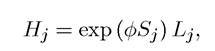
where Lj is employment in country j and φ is the rate on returns to schooling estimated from eq.
(3.25). This approach may not lead to very good estimates of the stock of human capital of a country, however. First, it does not take into account differences in other “human capital” factors, such as training or experience (which will be discussed in greater detail in Chapter 10). Second, countries may differ not only in the years of schooling of their labor forces, but in the quality of schooling and the amount of post-schooling human capital. Third, the rate of return to schooling may vary systematically across countries (for example, it may be lower in countries with a greater abundance of human capital). It is possible to deal with each of these problems to some extent by constructing better estimates of the stocks of human capital.Following Hall and Jones, let us make only a partial correction for the last factor. Let us assume that the rate of return to schooling does not vary by country, but is potentially different for different years of schooling. For example, one year of primary schooling may be more valuable than one year of graduate school (for example, because learning how to read might increase productivity more than a solid understanding of growth theory). In particular, let the rate of return to acquiring the Sth year of schooling be φ (S). The above equation would be the special case where φ (S) = φ for all S. With this assumption and with estimates of the returns to schooling for different years (e.g., primary schooling, secondaary schooling, and so on), a somewhat better estimate of the stock of human capital can be constructed as 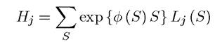 where
where now refers to the total employment of workers with S years of schooling in country j.
A series for Kj (t) can be constructed from the Summers-Heston dataset using investment data and the perpetual inventory method.
In particular, recall that, with exponential depreciation, the stock of physical capital evolves according to
where Ij (t) is the level of investment in country j at time t. The perpetual inventory method involves using information on the depreciation rate, δ, and investments, Ij (t)’s, to estimate Kj (t). Let us assume, following Hall and Jones that δ = 0.06. With a complete series for Ij (t), this equation can be used to calculate the stock of physical capital at any point in time. However, the Summers-Heston dataset does not contain investment information before the 1960s. This equation can still be used by assuming that each country’s investment was growing at the same rate before the sample in order to compute the initial capital stock. Using this assumption, Hall and Jones calculate the physical capital stock for each country in the year 1985. I do the same here for various years. Finally, with the same arguments as before, I choose a value of 1/3 for α.
Given series for Hj and Kj and a value for α, we can construct “predicted” incomes at a point in time using the following equation 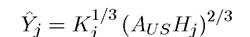
for each country j, where Aus is the labor-augmenting technology level of the United States, computed so that this equation fits the United States perfectly- Throughout, time indices are dropped.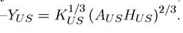
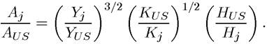
Once a series for Yj has been constructed, it can be compared to the actual output series. The gap between the two series represents the contribution of technology. Alternatively, we could explicitly back out country-specific technology terms (relative to the United States) as
Figures 3.3 and 3.4 show the results of these exercises for 1980, 1990 and 2000. The following features are noteworthy:
(1) Differences in physical and human capital still matter a lot; the predicted and actual incomes are highly correlated.
Thus the regression analysis was not entirely misleading in emphasizing the importance of physical and human capital.(2) However, differently from the regression analysis, this exercise shows that there are significant technology (productivity) differences. There are often large gaps between predicted and actual incomes, showing the importance of technology differences across countries. This can be most easily seen in Figure 3.3, where practically all observations are above the 45o, which implies that the neoclassical model is over predicting the income level of countries that are poorer than the United States.
(3) The same pattern is visible in Figure 3.4, which plots the estimates of the technology differences, Aj/Aus, against log GDP per capita in different years. These differences
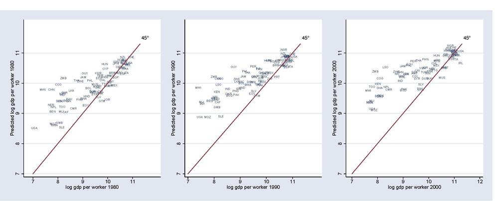
Figure 3.3. Calibrated technology levels relative to the US technology (from the Solow growth model with human capital) versus log GDP per worker, 1980, 1990 and 2000.
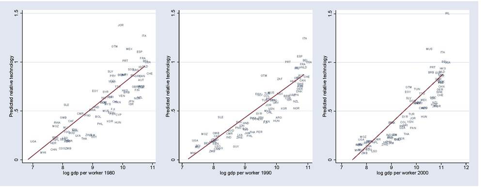
Figure 3.4. Calibrated technology levels relative to the US technology (from the Solow growth model with human capital) versus log GDP per worker, 1980, 1990 and 2000.
are often substantial. More important, these differences are also strongly correlated with income per capita; richer countries appear to have “better technologies”.
(4) Also interesting is the pattern that the empirical fit of the neoclassical growth model seems to deteriorate over time. In the Figure 3.3, the observations are further above the 45o in 2000 than in 1980, and in Figure 3.4, the relative technology differences become larger over time. Why the fit of the simple neoclassical growth model is better in 1980 than in 2000 is an interesting and largely unanswered question.
3.5.2. Challenges. In the same way as the regression analysis was based on a number of stringent assumptions (in particular, the assumption that technology differences across countries were orthogonal to other factors), the calibration approach also relies on certain important assumptions.
The above exposition highlighted several of those. In addition to the standard assumption that factor markets are competitive, the calibration exercise had to assume no human capital externalities, impose a Cobb-Douglas production function, and also make a range of approximations to measure cross-country differences in the stocks of physical and human capital.Let us focus on the functional form assumptions. Could we get away without the Cobb- Douglas production function? The answer is yes, but not perfectly. The reason for this is that the exercise here is very similar to growth accounting, which does not need to make strong functional form assumptions (and this similarity to growth accounting is the reason why this exercise is sometimes referred to as “levels accounting”). In particular, recall eq. (3.5), which showed how TFP estimates can be obtained from a general constant returns to scale production function (under competitive labor markets) by using average factor shares. Now instead imagine that the production function that applies to all countries in the world is given by
and countries differ according to their physical and human capital as well as technology—but not according to F. Suppose also that we have data on Kj and Hj as well as capital and labor share for each country. Then, a natural adaptation of eq. (3.5) can be used across countries rather than over time. In particular, let us a rank countries in descending order according to their physical capital to human capital ratios, Kj/Hj (use Exercise 3.1 to think about why this is the right way to rank countries rather than doing so randomly). Then,
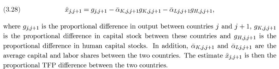
Using this method, and taking one of the countries, for example the United States, as the base country, we can calculate relative technology differences across countries.
This levels accounting exercise faces two major challenges, however. One is data-related and the other one theoretical. First, data on capital and labor shares across countries are not available for most countries. This makes the use of eq. (3.28) far from straightforward. Consequently, almost all calibration or levels accounting exercises that estimate technology (productivity) differences use the Cobb-Douglas approach of the previous subsection (a constant value of ακ equal to 1/3).Second, even if data on capital and labor shares were available, the differences in factor proportions, e.g., differences in across countries are large. An equation like (3.28) is a good approximation for small (infinitesimal) changes. As illustrated in Exercise 3.1, when differences in factor proportions are significant between the two observations, the use of this type of equation can lead to significant biases.
To sum up, the approach of calibrating productivity differences across countries is a useful alternative to the regression analysis, but has to rely on a range of stringent assumptions on the form of the production function and can also lead to biased estimates of technology differences when factors are mismeasured.
3.6.