Estimating Productivity Differences
In the previous section, productivity/technology differences are obtained as “residuals” from a calibration exercise, so we have to trust the functional form assumptions used in this strategy.
But if we are willing to trust the functional forms, we can also estimate these differences econometrically rather than rely on calibration. The great advantage of econometrics relative to calibration is that not only do we obtain estimates of the ob jects of interest, but we also have standard errors, which show us how much we can trust these estimates. In this section, I briefly discuss two different approaches to estimating productivity differences.3.6.1. A Naive Approach. The first possibility is to take a production function of the form (3.27) as given and try to estimate this using cross country data. In particular, taking logs:
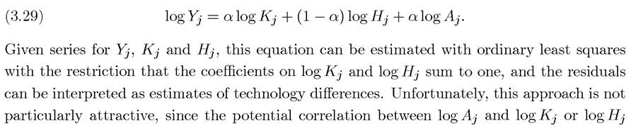
implies that the estimates of α need not be unbiased even when constant returns to scale is imposed. Moreover, if we do not impose the assumption that these coefficients sum to one and test this restriction, it will be rejected. Thus, this regression approach runs into the same difficulties as the Mankiw, Romer and Weil approach discussed previously.
What this discussion highlights is that, even if we are willing to presume that we know the functional form of the aggregate production function, it is difficult to directly estimate productivity differences. So how can we improve over this naive approach? The answer involves making more use of economic theory. Estimating an equation of the form (3.29) does not make use of the fact that we are looking at the equilibrium of an economic system. A more sophisticated approach would use more of the restrictions imposed by equilibrium behavior (and bring additional relevant data).
I next illustrate this using a specific attempt based on international trade. The reader who is not familiar with trade theory may want to skip this subsection.3.6.2. Learning from International Trade*. Models of growth and international trade are studied in Chapter 19. Even without a detailed discussion of international trade theory, we can use data from international trade flows and some simple principles of international trade theory to obtain another way of estimating productivity differences across countries.
Let us follow an important paper by Trefler (1993), which uses an augmented version of the standard Heckscher-Ohlin approach to international trade. The Heckscher-Ohlin approach assumes that countries differ according to their factor proportions (e.g., some countries have much more physical capital relative to their labor supply than others). In a closed economy, this will lead to differences in relative factor costs and differences in the relative prices of products using these factors in different intensities. International trade results as a way of taking advantage of these relative price differences. The most extreme form of the theory assumes no costs of shipping goods and no policy impediments to trade, so that international trade can happen costlessly between countries.
Trefler starts from the standard Heckscher-Ohlin model of international trade, but allows for factor-specific productivity differences, so that capital in country j has productivity thus a stock of capital Kj in this country is equivalent to an effectivesupply of capital
 Similarly for labor (human capital), country j has productivity
 In addition, Trefler assumes that all countries have the same homothetic preferences and there are sufficient factor intensity differences across goods to ensure international trade between countries to arbitrage relative price and relative factor costs differences (or in the jargon of international trade, countries are said to be in the cone of diversification).
Under these assumptions, a standard equation in international trade links the net factor exports of each country to the abundance of that factor in the country relative to the world as a whole. The term “net factor exports” needs some explanation. It does not refer to actual trade in factors (such as migration of people or capital flows). Instead trading goods is a way of trading the factors that are embodied in that particular good. For example, a country that exports cars made with capital and imports corn made with labor is implicitly exporting capital and importing labor. More specifically, the net export of capital by country is calculated by looking at the total exports of country j and computing how much capital is necessary to produce these and then subtracting the amount of capital necessary to produce its total imports. For our purposes here, how this is calculated is not important (it suffices to say that as with all things empirical, the devil is in the detail and these calculations are far from straightforward and require a range of assumptions). Then, the absence of trading frictions across countries and identical homothetic preferences imply that
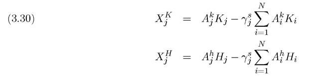
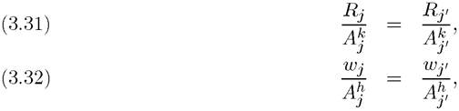
where is the share of country j in world consumption (the value of this country’s consumption divided by world consumption) and N is the total number of countries in the world. These equations simply restate the conclusion in the previous paragraph that a country will be a net exporter of capital if its effective supply of capital,
 exceeds a fraction, here
  of the world’s effective supply of capital,
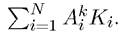
Consumption shares are easy to calculate.
Then, given estimates for and
and , the above system of 2 ? N equations can be solved for the same number of unknowns, the
 and
and for N countries. This gives estimates for factor-specific productivity differences across countries, generated from an entirely different source of variation than those exploited before. In fact, this exercise provides us with not a single productivity parameter, but a separate labor-augmenting (or human-capital-augmenting) and a capital-augmenting productivity term for each country.
 How do we know that these numbers provide a good approximation to cross-country factor productivity differences? This is in some sense the same problem as we had in judging whether the calibrated productivity (technology) differences in the previous section were reliable. Fortunately, international trade theory gives us one more set of equations to check whether these numbers are reliable. As noted above, under the assumption that the world economy is sufficiently integrated, there is conditional factor price equalization. This implies that for any two countries j and j0:
where Rj is the rental rate of capital in country j and Wj is the observed wage rate (which includes the compensation to human capital) in country j. Equation (3.32), for example, states that if workers in a particular country have, on average, half the efficiency units as those in the United States, their earnings should be roughly half of American workers.
With data on factor prices, we can therefore construct an alternative series for and
and  It turns out that the series for
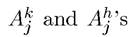 implied by (3.30), (3.31) and (3.32) are
very similar, so there appears to be some validity to this approach.
This validation gives us some confidence that there is some information in the numbers that Trefler obtains.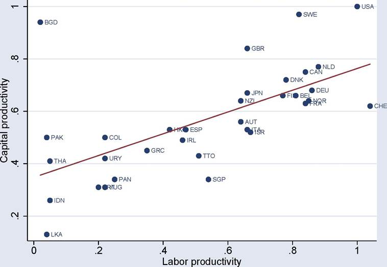
Figure 3.5. Comparison of labor-productivity and capital-productivity differences across countries.
Figure 3.5 shows Trefler’s original estimates. The numbers in this figure imply that there are very large differences in labor productivity, and some substantial, but much smaller differences in capital productivity. For example, labor in Pakistan is 1∕25th as productive as labor in the United States. In contrast, capital productivity differences are much more limited than labor productivity differences; capital in Pakistan is only half as productive as capital in the United States. This finding is not only intriguing in itself, but is also quite consistent with models of directed technological change in Chapter 15 that may explain why technological change is labor-augmenting in the long run.
It is also informative to compare the productivity difference estimates from Trefler’s approach to those from the previous section. Figures 3.6 and 3.7 undertake this comparison. The first plots the labor-productivity difference estimates from the Trefler approach against the calibrated overall productivity differences from the Cobb-Douglas specification in the previous section. The similarity between the two series is remarkable. This gives us some confidence that both approaches are capturing some features of reality and that in fact there are significant productivity (technology) differences across countries. Interestingly, however, Figure 3.7 shows that the relationship between the calibrated productivity differences and the capital-productivity differences is considerably weaker than for labor productivity.
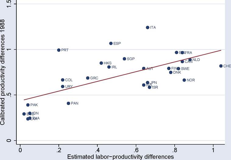
Figure 3.6. Comparison of the labor productivity estimates from the Trefler approach with the calibrated productivity differences from the Hall-Jones approach.
Despite its apparent success, it is important to emphasize that Trefler’s approach relies on very stringent assumptions. To recap, the three major assumptions are:
(1) No international trading costs;
(2) Identical homothetic preferences;
(3) Sufficiently integrated world economy, leading to conditional factor price equalization.
All three of these assumptions are rejected in the data in one form or another. There are clearly international trading costs, including freight costs, tariff costs and other trading restrictions. There is very well-documented home bias in consumption violating the identical homothetic preferences assumption. Finally, most trade economists believe that conditional factor price equalization is not a good description of factor price differences across countries. In view of all of these, the results from the Trefler exercise have to be interpreted with caution. Nevertheless, this approach is important in showing how different sources of data and additional theory can be used to estimate cross-country technology differences and in providing a cross-validation for the calibration and estimation results discussed previously.
Figure 3.7. Comparison of the capital productivity estimates from the Tre- fler approach with the calibrated productivity differences from the Hall-Jones approach.
3.7.