Growth Accounting

As discussed in the previous chapter, at the center of the Solow model is the aggregate production function, (2.1), which I rewrite here in its general form:

Another major contribution of Bob Solow to the study of economic growth was the observation that this production function, combined with competitive factor markets, also gives us a framework for accounting for the sources of economic growth.

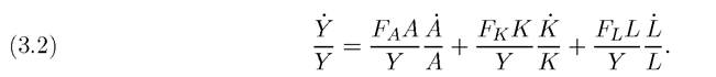
For our purposes, it is sufficient to expose the simplest version of this framework. Consider a continuous-time economy and differentiate the production function (3.1) with respect to time. Dropping time dependence and denoting the partial derivatives of F with respect to

its arguments by Fa, Fk and Fl, this yields

Now denote the growth rates of output, capital stock and labor by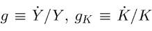 and gL ? L/L, and also define

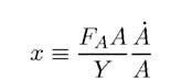
as the contribution of technology to growth. Next, recall from the previous chapter that with competitive factor markets, we have w = Fl and R = Fk (eq.’s (2.6) and (2.7)) and define the factor shares as ακ ? RK/Y and ¾ ? wL/Y. Putting all these together, (3.2) can be written as

This is the fundamental growth accounting equation. At some level it is no more than an identity. However, it also allows us to estimate the contribution of technological progress to economic growth using data on factor shares, output growth, labor force growth and capital stock growth.

In particular, denoting an estimate by “^ë”, we have the estimate of TFP growth at time t as:

I only put the “^ë” on x, but one may want to take into account that all of the terms on the right-hand side are also “estimates” obtained with a range of assumptions from national accounts and other data sources.

In addition, if the production function takes the standard labor-augmenting form Y (t) = 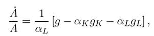but this equation is not particularly useful, sinceis not something we are inherently interested in. The economically interesting object is in fact X in (3.4), since it directly measures the effect of technological progress on output growth.

In continuous time, eq. (3.4) is exact because it is defined in terms of instantaneous changes (derivatives). In practice, instead of instantaneous changes, we look at changes over discrete time intervals, for example over a year (or sometimes with better data, over a quarter or a month). With discrete time intervals, there is a potential problem in using (3.4); over the time horizon in question, factor shares can change; should we use beginning-of-period or end-of-period values of ακ and Ol ? It can be shown that the use of either beginning-of-period or end-of-period values might lead to seriously biased estimates of the contribution of TFP to output growth, X. This is particularly likely when the distance between the two time periods 84

is large (see Exercise 3.1). The best way of avoiding such biases is to use as high-frequency data as possible.

For now, taking the available data as given, let us look at how one could use the growth accounting framework with data over discrete intervals. The most common way of dealing with the problems pointed out above is to use factor shares calculated as the average of the beginning of period and end of period values. Therefore in discrete time, for a change between times t and t + 1, the analog of eq. (3.4) becomes

where g⅛ t₊ι is the growth rate of output between t and t + 1, and other growth rates are defined analogously. Moreover,

are average factor shares between t and t +1. Equation (3.5) would be a fairly good approx­imation to (3.4) when the difference between t and t + 1 is small and the capital-labor ratio does not change much during this time interval.

Solow’s (1957) article not only developed this growth accounting framework but also applied it to US data for a preliminary assessment of the “sources of growth” during the early 20th century. The question Bob Solow asked was this: how much of the growth of the US economy can be attributed to increased labor and capital inputs, and how much of it is due to the residual, “technological progress”? Solow’s conclusion was quite striking: a large part of the growth was due to technological progress.

This has been a landmark finding, emphasizing the importance of technological progress as the driver of economic growth not only in theory, but also in practice. It focused the attention of economists on sources of technology differences over time, and across nations, industries and firms.

From early days, however, it was recognized that calculating the contribution of technolog­ical progress to economic growth in this manner has a number of pitfalls. Moses Abramovitz (1956), famously, dubbed the X term “the measure of our ignorance”—after all, it was the residual that we could not explain and we decided to call it “technology”.

In its extreme form, this criticism is unfair, since X does correspond to technology ac­cording to eq. (3.4); thus the growth accounting framework is an example of using theory to inform measurement. Yet at another level, the criticism has validity. If we mismeasure the growth rates of labor and capital inputs, g∣. and gκ, we will arrive at inflated estimates of X. And in fact there are good reasons for suspecting that Solow’s estimates and even the higher-quality estimates that came later may be mismeasuring the growth of inputs. The most obvious reason for this is that what matters is not labor hours, but effective labor hours, so it is important—though difficult—to make adjustments for changes in the human capital of workers. I discuss issues related to human capital in Section 3.3 below and then in greater detail in Chapter 10. Similarly, measurement of capital inputs is not straightforward. In the theoretical model, capital corresponds to the final good used as input to produce more goods. But in practice, capital is machinery, and in measuring the amount of capital used in production one has to make assumptions about how relative prices of machinery change over time. The typical assumption, adopted for a long time in national accounts and also naturally in applications of the growth accounting framework, was to use capital expendi­tures. However, if the same machines are much cheaper today than they had been in the past (as has been the case for computers, for example), then this methodology would severely underestimate gκ (recall Exercise 2.23 in the previous chapter). Therefore, when applying eq. (3.4), underestimates of gr and gκ will naturally inflate in the estimates of the role of technology as a source of economic growth.

What the best way of making adjustments to labor and capital inputs in order to arrive to the best estimate of technology is still a hotly debated area. Dale Jorgensen, for example, has shown that the “residual” technology can be reduced very substantially (perhaps almost to 0) by making adjustments for changes in the quality of labor and capital (see, for example, Jorgensen, Gollop and Fraumeni, 1987, or Jorgensen, 2005). These issues will also become relevant when we attempt to decompose the sources of cross-country output differences. Before doing this, let us look at applications of the Solow model to data using regression analysis.

3.2.