Externalities from Capital Accumulation and Economic Growth

We start with a class of models in which physical capital accumulation leads to improved labor efficiency through a process of learning by doing. It is assumed in these models that the accumulation of aggregate capital implies a direct externality that leads to higher efficiency of labor, as a higher aggregate capital stock implies a higher stock of accumulated experience of all workers in the production process.

In this class of models, capital has both direct effects on labor productivity and also indirect effects through the accumulated economywide efficiency of workers. The indirect impact of capital accumulation on labor efficiency is an example of a positive externality. Knowledge spillovers, which are a positive function of the aggregate capital stock, increase the efficiency of labor. It is assumed here that knowledge is like a public good and that the accumulation of knowledge depends on the accumulation of aggregate capital.

8.1.1 Definitions

The definitions of the variables are analogous to those we have used in previous models. However, the efficiency of labor is now an endogenous variable that depends on the accumulation of physical capital. We thus define: Y, aggregate output (or ŷ, output per worker); K, aggregate (physical) capital stock (or , capital per worker); h, efficiency of labor, or “human capital” per worker (an endogenous variable that depends on the accumulation of aggregate capital per worker); C, aggregate consumption (or ĉ, consumption per worker); r, real interest rate; and ŵ, real wage per worker.

The exogenous variables and exogenous parameters in the model are defined as follows: t, time (a discrete exogenous variable); L, population and labor force (an exogenous variable that depends on time); n, rate of growth of population (exogenous parameter); g, rate of technical progress (exogenous parameter); δ, rate of depreciation of capital (exogenous parameter); ρ, pure rate of time preference of households (exogenous parameter); s the savings rate (in the Solow model); α, the exponent of capital in a Cobb-Douglas production function; and A, total factor productivity.

8.1.2 The Production Function

Production of goods and services takes place through a large number of competitive firms. The production function of firm i is given by

The production function is characterized by constant returns to scale and satisfies the usual conditions of a neoclassical production function. We can thus write the production function as

where ŷ_i = Y_i/L_i is output per worker of firm i; is physical capital per worker of firm i; and h is efficiency of labor, or human capital per worker in firm i, assumed to be the same for all firms.

In what follows we assume a Cobb-Douglas production function of the form

where 0 < α < 1 is the direct elasticity of output with respect to the capital stock, and A is total factor productivity. Those two parameters, as well as the efficiency of labor h, are assumed to be the same for all firms.

8.1.3 Externalities from the Accumulation of Capital

Unlike the growth models we have analyzed so far, where labor augmenting technical progress was assumed exogenous, we will assume that the aggregate efficiency of labor is a function of both time and the aggregate capital stock per worker in the economy. This dependence is justified on the basis of the learning by doing concept of Arrow [1962]. Economies with a high capital stock per worker are characterized by higher labor efficiency as well, because of the accumulated experience of workers in the production process.

As noted by Arrow [1962, p. 156],

I advance the hypothesis here that technical change in general can be ascribed to experience, that it is the very activity of production which gives rise to problems for which favorable responses are selected over time.

Thus, on the basis of this observation, assume that the efficiency of labor is determined by

where 0 ≤ β ≤ 1. K is the aggregate capital stock (an index of experience), and L is aggregate employment of labor. From (8.4), a higher aggregate capital stock per worker implies a higher efficiency of labor for all workers in the economy, irrespective of the capital stock used by the firm that employs the particular worker. The parameter β measures the elasticity of labor efficiency with respect to the aggregate capital stock per worker, and g is the exogenous rate of technical progress.

Substituting (8.4) in (8.3) and aggregating the production of all firms, we can derive the aggregate production function:

From (8.5), it follows that aggregate output per worker is given by

where ŷ = Y/L and = K/L.

The shape of this production function is depicted in figure 8.1 for different values of the parameter β. For β = 0, there is no effect of the aggregate accumulation of capital on labor efficiency, and we are back to an aggregate Cobb-Douglas production function without externalities. The efficiency of labor depends only on the exogenous rate of technical progress g.

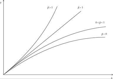
Figure 8.1 The aggregate production function for different values of β.

In the case β < 1, the properties of the exogenous-growth models we have analyzed so far do not change by much. There are decreasing returns to capital accumulation, and the economy converges to a balanced growth path that can be analyzed in the same way as the exogenous-growth models in previous chapters. However, if β ≥ 1, then (8.6) leads to endogenous growth.

In what follows, we concentrate on the special case β = 1, which implies endogenous growth without violating the assumption of constant returns to scale. In the special case β = 1, (8.5) and (8.6) take the form

where (8.8) implies that aggregate output per worker is a linear function of capital per worker. The marginal and average productivity of capital is constant. Because of the linearity of the aggregate production function, the rate of growth of output per worker (or per capita income) g is equal to the rate of growth of capital per worker.

where g is now endogenous and is determined by the rate of accumulation of capital.

For the same reason, from (8.7), the rate of growth of aggregate output g + n is determined by the share of net investment in total output. As a result, we have that

where I denotes gross investment in physical capital, and δ is the depreciation rate.²

8.1.4 Determination of the Real Interest Rate and the Real Wage

Assuming that firms operate under perfect competition, they maximize profits by taking the prices of inputs as given. Profit maximization implies that the real interest rate will be equal to the marginal product of capital for individual firms, and the real wage will equal the marginal product of labor for individual firms. From the point of view of each individual firm, the efficiency of labor is exogenously given. Thus, from (8.3), the net marginal product of capital for each individual firm is given by

Substituting h(t) from (8.4) and assuming that β = 1, we get the marginal productivity condition

where r(t) is the real interest rate, and the expression on the right-hand side is the net marginal product of capital from the vantage point of each individual firm. Equation (8.11) implies that all firms will select the same capital per worker, as they face the same real interest rate and the same labor efficiency per worker. Therefore, .

The real interest rate is constant and equal to the private marginal product of capital, as calculated by each individual firm. Because of its small size, each competitive firm does not internalize the effects of its own choice of capital per worker on the aggregate capital stock per worker in the economy, treating labor efficiency as exogenously given. Labor efficiency depends on the aggregate capital stock per worker and not on the firm-specific capital per worker. This externality explains why each firm underestimates the social marginal product of capital and why the real interest rate, as determined in competitive markets, is lower than the social (aggregate) marginal product of capital. We shall return to this market failure in section 8.1.7 below, when we discuss the efficiency of the competitive equilibrium.³

In competitive equilibrium, the real wage will be equal to the marginal product of labor as calculated by each individual firm. It is thus determined by

where ŵ(t) is the real wage per worker, and the property that in the competitive equilibrium , ∀i has been used.

The real wage is a constant share of output per worker. If output per worker is growing at a rate g, then the real wage per worker will also be growing at a rate g.

Note that this endogenous-growth model predicts a constant real interest rate and growing real wages per worker, in agreement with the Kaldor stylized facts analyzed in chapter 3.

However, unlike the exogenous-growth models we have analyzed so far, this model does not predict convergence. As we shall see, the growth rate is constant and endogenously determined. Therefore, two economies that have different initial capital stocks per worker will not experience convergence to the same per capita output and income, even if they have the same technological and population parameters and the same preferences of consumers. They will have the same endogenous growth rate, but conditional convergence does not occur in such an endogenous-growth model.⁴

8.1.5 The Savings Rate and the Endogenous Growth Rate

Let us first assume that, as in the Solow model, consumer behavior is described by a constant savings rate. Per capita consumption is thus given by

where s is the exogenous savings rate.

In equilibrium, total output will be equal to consumption plus gross investment. In per capita terms, we have

Combining (8.8), (8.14), and (8.15), the change in the capital stock per worker will be given by

Dividing both sides of (8.16) by (t), we get

Equation (8.17) determines the endogenous growth rate g. The higher the exogenous savings (and investment) rate s and total factor productivity A are, the higher the growth rate of per capita income will be. However, population growth and the depreciation rate have a negative impact on the endogenous growth rate.

In this model, the savings rate plays a similar role to its role in the exogenous-growth Solow model. In the latter model, the savings rate has a positive impact on steady state capital k^* and output per effective unit of labor y^*, and the transitional growth rate during the convergence process toward the steady state, but it does not affect the long-term growth rate, which is equal to the exogenous rate of technical progress g. In this endogenous-growth Arrow-Romer-Solow model, with positive externalities from capital accumulation, the savings rate s determines the gross investment rate (and through the gross investment rate, the endogenous growth rate), because the accumulation of capital does not imply diminishing returns for the marginal product of capital, and growth continues forever.

Therefore, in this endogenous-growth model, economies characterized by different stocks of initial capital will not converge to the same per capita income, even if they have identical savings rate, total factor productivity, rate of population growth, and depreciation rate. They will simply have the same steady state growth rate, without converging to the same per capita income on the balanced growth path. Their initial differences will be maintained forever.

8.1.6 Externalities and Endogenous Growth in the Ramsey Model

As already mentioned, the assumption of an exogenous savings rate is not theoretically satisfactory. The savings rate is determined by underlying factors associated with the preferences and constraints of households.

How is the endogenous growth determined in a representative household model, where households maximize the intertemporal utility from consumption? Assume a representative household, which maximizes the intertemporal utility function

subject to the household budget constraint

Variables in (8.18) and (8.19) are defined per capita. Income per capita is capital income per capita plus labor income per capita. Each household member supplies one unit of labor.

From the first-order conditions for a maximum, we get the Euler equation for consumption (see chapter 4):

Given that the real interest rate is constant and equal to αA − δ, from (8.12), the rate of growth of per capita consumption is also constant and is given by

This determines the endogenous growth rate g, as on a balanced growth path, all per capita variables grow at the same rate. If that were not so, either consumption or investment would eventually grow to be equal to output.

From (8.21), a higher pure rate of time preference of households, relative to the private marginal product of capital to firms (the real interest rate), results in a lower endogenous growth rate of per capita income and consumption. This is because a higher pure rate of time preference of households implies lower savings and a lower rate of accumulation of capital. In contrast, a higher total factor productivity A or a higher private contribution of capital to output α leads to a higher endogenous growth rate, as both result in a higher equilibrium real interest rate and higher savings and capital accumulation rates. For the opposite reason, the depreciation rate δ has a negative impact on the endogenous growth rate.

To find the savings rate, we use (8.8) and (8.15). These equations imply that

Equation (8.22) is the aggregate equilibrium condition of equality of total output to consumption plus investment. Dividing through by (t) yields

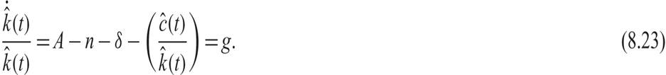
From (8.23) it follows that

From (8.24) and the aggregate production function (8.8), the share of consumption to total output is equal to

From (8.25) and (8.21), the aggregate savings rate is equal to

The savings rate in this endogenous-growth Ramsey model is constant, because the real interest rate is constant. It depends positively on the determinants of the real interest rate αA − δ, the rate of population growth n, and the elasticity of intertemporal substitution in consumption 1/θ, and negatively on the pure rate of time preference of households ρ. The effect of the depreciation rate of capital on the endogenous savings rate depends on the elasticity of intertemporal substitution in consumption. If the latter is equal to one, which implies θ = 1, then the depreciation rate of capital has no effect on the savings rate. If the elasticity of intertemporal substitution in consumption is greater than one (θ < 1), then the depreciation rate of capital has a negative effect on the savings rate. The opposite happens if the elasticity of intertemporal substitution is less than one (θ > 1).

These effects are analogous to the steady state effects in the Ramsey exogenous-growth model. The main difference in the Arrow-Romer-Ramsey endogenous-growth model has to do with the determinants of the endogenous growth rate in (8.21) and the fact that there is no conditional convergence in this model. Another difference is that, because of the existence of positive externalities in the Arrow-Romer-Ramsey model, the competitive equilibrium is socially suboptimal, as it does not maximize social welfare.

8.1.7 The Suboptimality of the Competitive Equilibrium with Externalities Due to Capital Accumulation

In chapter 4, we have already demonstrated that in the exogenous-growth Ramsey model without externalities, the competitive equilibrium maximizes social welfare. Does this result carry over to the Ramsey model with externalities from capital accumulation, as in the endogenous-growth model we have analyzed? The existence of externalities would immediately suggest that the answer is no.

To examine the nature of the suboptimality of the competitive equilibrium, let us assume there is a social planner who maximizes (8.18) under the macroeconomic constraint (8.22) instead of the private constraint (8.19). From the first-order conditions for a maximum, the Euler equation for the social planner would take the form

From the above inequality, we can deduce that the endogenous growth rate in the competitive economy is lower than the socially efficient growth rate. This is because the competitive real interest rate (αA − δ) underestimates the social net marginal product of capital (A − δ), which, because of the positive externality from capital accumulation, is higher than the private net marginal product of capital. Because the positive externality from capital accumulation is not reflected in the real interest rate, households have a smaller incentive to save and accumulate capital, and, as a result, the savings rate, the investment rate, and the growth rate of the economy are lower than what would be socially optimal.

Thus, the competitive equilibrium is suboptimal and could be improved on by a social planner who would choose savings and capital accumulation, taking the externality into account. Various other policies, such as the subsidization of capital, could improve efficiency in this case.

Exercise 8.1 Assume a competitive representative household model in which the production technology is as in (8.5), with 0 < β < 1. Derive the steady state, and discuss the properties of the steady state and the adjustment path. How does the steady state compare with the steady state of a model without externalities from learning by doing? Is the speed of adjustment higher or lower, and how does it depend on the strength of the externalities from capital accumulation? What determines the long-run growth rate in this model? Discuss the optimality properties of the competitive equilibrium.

8.1.8 Externalities and Endogenous Growth in the Blanchard-Weil Model

We next turn to the determinants of endogenous growth in an OLG model with externalities from capital accumulation. We shall utilize the Blanchard-Weil model, where population growth comes from the entry of new households. The number of members of each household is constant, and the rate of entry of new households is equal to n. Every household has an infinite time horizon.

The household born at instant j maximizes the intertemporal utility function

where c( j, t) is consumption at instant t of the household born at instant j, u is the instantaneous utility function of the household, and ρ is pure rate of the time preference of the household.

Following Blanchard [1985] and Weil [1989], we shall assume that the instantaneous utility function is logarithmic:

All households supply one unit of labor and receive a real wage ŵ, and to the extent that they have accumulated savings, they also receive capital income. Household j thus maximizes (8.27) under the constraint

where k( j, j) = 0.

From the first-order conditions, and after aggregation, we get the following equation for the evolution of aggregate consumption:⁵

From (8.30), after division by L(t), the evolution of per capita consumption is described by

Dividing (8.31) by per capita income ŷ(t), and after replacing the real interest rate from (8.12) and the capital output ratio from (8.8), we get the following equation for the evolution of the ratio of private consumption to total output:

where for any variable X, we define its ratio to total output Y as

From the per capita capital accumulation equation (8.22), we get

Equation (8.33) suggests that the aggregate growth rate g + n is equal to the net savings (=investment) rate times total factor productivity, minus the depreciation rate. Because of constant returns to capital accumulation, total factor productivity is equal to the (constant) average and marginal product of capital.

From (8.32) and (8.33), we can determine the two endogenous variables, that is, the growth rate and the savings rate. Given that neither is a predetermined variable, the equilibrium is achieved instantaneously.

For a constant ratio of private consumption to output, (8.32) implies

The higher the growth rate is, the greater will be the ratio of private consumption to total output for a given difference between the real interest rate and the pure rate of time preference of households.

Solving (8.33) and (8.34) for the endogenous growth rate, we get that

From (8.35), it follows that the endogenous growth rate in an Arrow-Romer-Blanchard-Weil model is lower than that in the corresponding Arrow-Romer-Ramsey model. The reason is that savings, and therefore capital accumulation and growth, are lower in the former model, because current generations do not internalize the welfare of future generations.

The difference between the two models can be depicted graphically, with the help of figure 8.2. The nonlinear relationship (8.34) between the consumption rate and the growth rate is represented by the positively sloped curve in figure 8.2. Obviously, as g tends to αA − δ − ρ, the ratio of private consumption to total income tends to infinity.

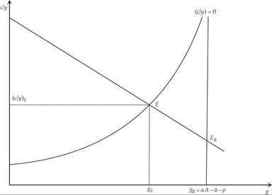
Figure 8.2 Determination of the consumption-to-output ratio and the endogenous growth rate in the Blanchard-Weil model.

The capital accumulation equation (8.33) is represented by the negatively sloped line. The higher the ratio of private consumption to total income is, the smaller will be the savings rate, the investment rate, and the endogenous growth rate.

The equilibrium is determined at the intersection of the two loci (point E in the figure). Because neither private consumption nor the rate of economic growth is a predetermined variable, the economy jumps directly to the equilibrium at E. Note that the equilibrium ratio of private consumption to output is greater than in the corresponding representative household model and the endogenous growth rate is lower. The equilibrium in the corresponding representative household model (n = 0) is determined at point E_R.

The Arrow-Romer-Blanchard-Weil model implies two externalities that reduce the long-run growth rate. One arises because current generations do not internalize the welfare of future generations and thus save less than would be socially optimal, and the second arises because firms do not internalize the effects of their capital stock decisions on the aggregate capital stock and hence on the efficiency of labor. The corresponding Arrow-Romer-Ramsey model implies only the latter of the two externalities.

8.1.9 Fiscal Policy and Endogenous Growth

When we introduce the government, the effects of fiscal policy are analogous to the effects in the exogenous-growth Blanchard-Weil model. The exogenous-growth version of the model determines the capital stock and consumption per efficiency unit of labor, whereas the endogenous-growth version determines the growth rate and the ratio of consumption to total output.

Assuming that the government stabilizes the government debt to output ratio and that it selects a fixed ratio of primary government expenditure to total output, the endogenous-growth Blanchard-Weil model takes the following form:

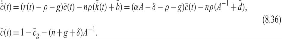
The top equation in (8.36) is the aggregate private consumption function, when households hold assets in both capital and government bonds, and is derived from (8.32). The bottom equation is derived from (8.33) with the addition of primary government expenditure; it describes the capital accumulation rate, which is equal to the endogenous growth rate, as a result of total domestic savings.

The additional assumption that the government selects a constant government debt and primary expenditure to output ratio takes the form

The model of (8.36) determines the ratio of private consumption to total output , and the growth rate g.

The equilibrium is depicted in figure 8.3. The dashed positively sloped curve depicts the top equation in (8.36), for a constant ratio of private consumption to total output, and is given by

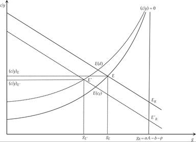
Figure 8.3 Determination of private consumption and the growth rate with government expenditure and debt.

The higher the growth rate is, the greater the ratio of private consumption to total output will be, for a given difference between the real interest rate and the pure rate of time preference of households. The nonlinear relationship is represented by the dashed upward-sloping curve in figure 8.3. As g tends to αA − δ − ρ, the ratio of private consumption to total output tends to infinity.

For a positive ratio of government debt to output, this curve lies above the corresponding curve for zero government debt (solid curve). Current households consider government debt as part of their wealth and thus consume more relative to income, because they know that part of the future taxes to finance government debt will be paid by future generations.

The dashed negatively sloped straight line represents the negative relationship between growth (capital accumulation) and the private consumption ratio, because the higher the ratio of private consumption to output is, the lower the ratio of savings and investment to total output will be. With a positive ratio of primary government expenditure to total output, this line is below the corresponding line for zero primary government expenditure.

It is evident that both the ratio of government debt to output and that of primary government expenditure to output have a negative impact on the endogenous growth rate g. The reason is that both government debt and primary government expenditure cause a reduction in total savings and capital accumulation and thus reduce the growth rate. The equilibrium with government expenditure and taxes is at point E′, which implies a lower growth rate.

Government debt causes an increase in private consumption by current generations, reducing the rate of accumulation of capital and the growth rate (point E(d) in figure 8.3). Primary government expenditure causes a decline in private consumption that is not fully offsetting, reducing total savings, the rate of capital accumulation, and the growth rate (point E(c_g) in figure 8.3). The combination of the two results in even greater reduction in the endogenous rate of economic growth.

In the corresponding representative household model (with n = 0), the rate of economic growth is not affected by the level of government debt and primary government expenditure. The endogenous growth rate is determined by the difference of the real interest rate of the pure rate of time preference (point E_R in figure 8.3). Primary government expenditure crowds out an equal amount of private consumption and thus does not affect aggregate savings. Government debt does not affect private consumption, as it is considered equivalent to the present value of future taxes for the representative household (point in figure 8.3).

Exercise 8.2 Analyze the impact of capital income taxation in the Ramsey and Blanchard-Weil endogenous-growth models. Assume logarithmic preferences and a Cobb-Douglas technology with learning by doing. How does a tax rate τ_κ on interest income affect the steady state growth rate? Assume in your analysis that government expenditure and public debt per head are constant, and that the government redistributes receipts from the capital income tax back to households in a lump sum fashion.

8.1.10 Convergence in Exogenous and Endogenous AK Growth Models

We have already seen that, unlike in exogenous growth models, in endogenous growth models of the AK variety (such as those examined in this section), there is no convergence process.

In exogenous growth models, any two economies characterized by the same parameters describing the technology of production, household preferences, and economic policy will converge to the same balanced growth path, even if they start from different initial conditions. In endogenous growth models, they will have the same endogenous growth rate, but they will not converge to the same per capita income. Their initial differences will remain forever.

The analysis of this difference is presented in figure 8.4, where it is assumed that two otherwise identical economies are characterized by different initial conditions. Economy 1 has initially less capital and output per worker in relation to economy 2. In terms of the production technology, the preferences of consumers, and fiscal policy, the two economies are identical.

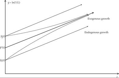
Figure 8.4 The path of per capita output in exogenous and endogenous growth models.

If the two economies are characterized by the conditions that apply to an exogenous growth model, then they both converge to the balanced growth path y^*(t). Initially, economy 1 will have a higher growth rate of output per head than economy 2. Gradually the two economies will converge to the balanced growth path y^*(t) and will be characterized by the same per capita output and the same growth rate of per capita output.

If the two economies are characterized by the conditions that apply to an endogenous growth model, then their initial differences will remain. Economies 1 and 2 will be characterized by the same rate of growth of per capita output, but their initial percentage differences in per capita output, per capita consumption, and real wages will persist. Economy 1 will follow the balanced growth path y₁(t), and economy 2 the balanced growth path y₂(t). Their per capita output, consumption, and real wages will grow at the same rate, but they will not converge.

The paths of per capita output of two such economies (in logarithms), under exogenous and under endogenous growth, are illustrated in figure 8.4.

Note that the available empirical evidence from postwar international experience indicates that conditional convergence cannot be dismissed easily, casting doubts on the applicability of endogenous growth models. However, this does not mean that externalities of the learning-by-doing variety do not exist, as such externalities are also compatible with exogenous growth models, as long as they do not lead to constant returns to the accumulation of physical capital.⁶

8.2