Investment in Human Capital and Economic Growth

In the learning-by-doing endogenous-growth model that we presented in the previous section, endogenous growth is essentially a by-product of the accumulation of physical capital, because it is assumed that labor efficiency is a function of the aggregate physical capital stock per worker.

An alternative class of growth models emphasizes the education and training of workers and the accumulation of human capital implied by such activities. In this section, we consider some alternative models in which the efficiency of labor depends on investment in human capital through education and training.

8.2.1 The Extended Solow Model and the Share of Spending on Education and Training

We start with a model in which the accumulation of human capital is the result of spending on education and training. The model is due to Mankiw et al. [1992] and is a generalization of the Solow model to allow for the accumulation of human as well as physical capital. The efficiency of labor depends partly on exogenous technical progress and partly on the stock of human capital, which accumulates due to investment in education and training.

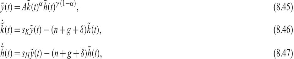
Firms are competitive, and their production technology is Cobb-Douglas, of the form

where 0 < α < 1, and ĥ(t) denotes the efficiency of labor at instant t.

Assume that the efficiency of labor is a function of human capital per worker h and exogenous technical progress. This function takes the form

where h is human capital per worker, resulting from accumulated education and training, and 0 ≤ γ ≤ 1 is a parameter that measures the relative contribution of human capital to the efficiency of labor.

Substituting (8.39) in (8.38), we get the following aggregate production function:

where H = hL is aggregate human capital.

We assume, generalizing the Solow model, that total household income is either consumed or invested in physical capital or invested in human capital. The percentage of output and income invested in physical capital equals s_K, and the percentage invested in human capital equals s_H. These percentages are considered exogenous, in the same way that the savings rate is assumed exogenous in the Solow model. Furthermore, assume that δ, the depreciation rate, is the same for both physical and human capital. With these assumptions, the accumulation equations for physical and human capital are given by

alt=eq8-41.png>

If γ = 0, then we get the familiar neoclassical production function, as spending on education and training does not contribute to labor efficiency of workers, which is a simple function of time (exogenous technical progress).

If 0 < γ < 1, we have a generalized model of exogenous growth, in which the per capita capital stock and output on the balanced growth path are positive functions of both the proportion of total income spent on physical capital accumulation s_K, and the proportion spent on education and training s_H.

In this case, the equilibrium condition in the goods and services market is given by

which, in conjunction with (8.41) and (8.42), implies a consumption function of the form

In the case where 0 < γ < 1, we can divide (8.40), (8.41), and (8.42) by the number of workers L times the exogenous labor efficiency e ^gt, and the model takes the form

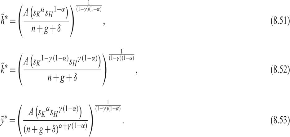
where 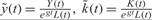, and .

8.2.2 The Balanced Growth Path in the Extended Solow Model

On the balanced growth path, all per capita variables grow at the rate of exogenous technical progress g. It therefore follows that

From (8.48), (8.49), and the production function (8.45), it follows that

From (8.50), it follows that on the balanced growth path, the ratio of physical to human capital is constant, and equal to the ratio of the investment rates in physical and human capital, respectively. This follows because equilibrium investment on the balanced growth path is a proportion n + g + δ of both physical and human capital, per exogenous efficiency unit of labor.

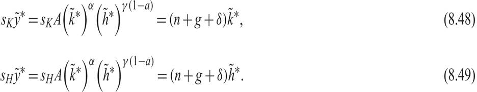
Substituting (8.50) in the production function and solving (8.48) and (8.49) results in

From (8.53), per capita output on the balanced growth path is given by

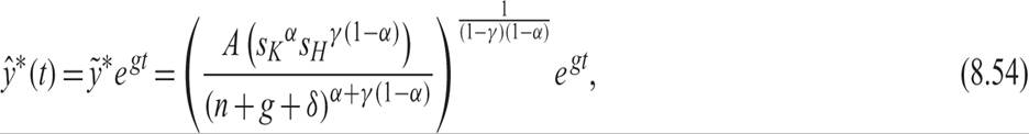
where .

The level of per capita output on the balanced growth path depends positively on total factor productivity A, the shares of output invested in physical and human capital (s_K and s_H), and negatively on the population growth rate n, the rate of exogenous technical progress g, and the depreciation rate δ. The growth rate of per capita output on the balanced growth path is equal to the rate of exogenous technical progress g.

Thus, in the case 0 < γ < 1, we have an extended Solow model of exogenous growth.

8.2.3 Endogenous Growth in the Extended Solow Model

If γ = 1 in (8.39), there is no exogenous technical progress. The efficiency of labor only depends on accumulated human capital. In this case, the model is an endogenous growth model. Setting γ = 1 in the production function (8.40) we get

where ŷ = Y/L, = K/L and ĥ = H/L.

In this model, the balanced growth path is defined by

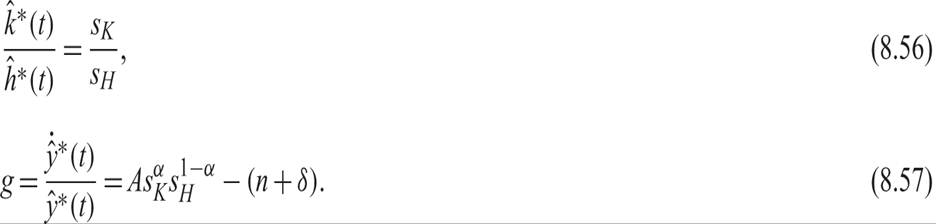
On the balanced growth path, the ratio of physical to human capital is stabilized at the ratio of the investment rates in physical and human capital. Because both physical and human capital are growing at the same rate, we have endogenous growth. The accumulation of physical capital causes an increase in income, which in turn causes an increase in human capital through expenditure on education and training. This in turn leads to a further rise in output, which causes new investment in physical capital. The parallel accumulation of physical and human capital leads to endogenous growth.

The endogenous growth rate depends positively on total factor productivity A and a weighted average of the income ratios invested in physical and human capital s_K and s_H. The growth rate of population n and the depreciation rate δ have a negative impact on the endogenous growth rate.

In all other respects, the properties of the endogenous growth, extended Solow model are similar to those of the learning-by-doing model of Arrow and Romer, as analyzed in section 8.1. The main difference is that in this extended Solow model, the accumulation of human capital is not a simple by-product of physical capital accumulation but the result of explicit investment on human capital through education and training.

8.2.4 The Jones Model of Human Capital Accumulation

We next consider an alternative model, in which human capital depends on the time span devoted to education and training. We assume that workers spend part of their time v in education and training and that this investment of time involves a rate of return ψ. The model is analyzed in Jones [2002].

The production technology is described by the production function (8.38). The efficiency of labor per employee is determined by

where the function h(v, ψ) determines human capital per worker as a function of the time span v devoted to education and training, and the rate of return of investment in human capital ψ.

A plausible form of this function is the exponential function. Let us therefore assume that

The exponential form is plausible, because it implies that the proportional change in the function with respect to the time devoted to education and training is equal to the rate of return ψ. From (8.59), we get

Substituting (8.59) in (8.58) and the resulting equation in the production function (8.38), we get that output per worker is determined by

Combining (8.61) with the savings assumption of the Solow model (i.e., that there is an exogenous constant savings rate), per capita output on the balanced growth path is determined by

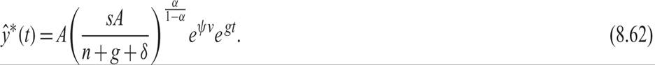
Per capita output on the balanced growth path is a positive function of the amount of time spent on education and training v and the rate of return on investment in human capital ψ. However, in all other respects, this model is an exogenous growth model, similar to the Solow model.

8.2.5 The Lucas Model of Human Capital Accumulation and Endogenous Growth

An alternative model of investment in human capital is the endogenous growth model of Lucas [1988], which is based in part on Uzawa [1965].

Lucas assumed that labor efficiency is equal to human capital per worker:

With regard to the production of human capital per worker, he assumed that this depends on the existing stock of human capital per worker times the proportion of nonleisure time that workers devote to education and training. He thus assumed that

According to (8.64), only human capital is required for the production of human capital. Here u is defined as the proportion of the nonleisure time of households that is devoted to the production of goods and services, and 1 − u is the proportion of time devoted to education and training. Education and training results in the accumulation of human capital. In addition, ζ is the productivity of human capital in the production of new human capital, n is the population growth rate, and δ the depreciation rate of human capital (assumed for simplicity to be equal to that of physical capital).

On the balanced growth path, u will be constant at u^*. Taking the integral of (8.64) and substituting in (8.63), we get

Lucas assumed that u is chosen by a representative household to maximize its intertemporal utility of consumption. As a result, the choice of u depends both on the preferences of the representative household and on the technological parameters characterizing the production of goods and services and human capital.

From the form of (8.65), it follows that the endogenous growth rate is equal to g = ζ(1 −u^*) − (n + δ), which works like the exogenous rate of technical progress in exogenous growth models. The higher is the steady state proportion of nonleisure time devoted to education and training, the higher the endogenous growth rate will be. In the Lucas model, 1 − u^* is chosen endogenously, and in conjunction with the exogenous ζ, δ, and n, it determines the steady state growth rate of per capita output.

8.2.6 A Detailed Analysis of the Lucas Model

In what follows, we proceed to analyze in detail the Lucas [1988] model. The dynamic analysis of this model has been generalized by Caballe and Santos [1993], Faig [1995], and Mulligan and Sala-i Martin [1993].

As in the Ramsey model, the representative household is assumed to maximize

subject to the following constraints:

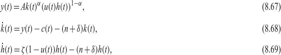
where c is consumption per capita, y is output per capita, k is the stock of physical capital per capita, h is the stock of human capital per capita, and u is the proportion of nonleisure time spent on the production of goods and services. Thus, 1 − u is the proportion of nonleisure time spent on the accumulation of human capital.

Equation (8.67) is the production function for goods and services, (8.68) the accumulation equation for physical capital, and (8.69) the accumulation equation (production function) for human capital. Let us assume constant returns to scale in both the goods and services sector and the human capital sector. Building on the model of Uzawa [1965], Lucas assumed that only human capital is used in the production of human capital.

In these equations, ρ is the pure rate of time preference of the representative household, 1/θ is the elasticity of intertemporal substitution in consumption, A is total factor productivity in the production of goods and services, α is the elasticity of output of goods and services with respect to physical capital, ζ is total factor productivity in the production of human capital, and δ is the depreciation rate of both types of capital.

From (8.69), the growth rate of human capital per worker is given by

On the balanced growth path, the growth rate of human capital per worker is constant and equal to the growth rate of all other per capita variables. Given that the growth rate is determined by u, to determine the growth rate, we must consider how the representative household selects it.

The current-value Hamilton function for the problem of the representative household takes the form

where we have omitted the time index and substituted out the production function of goods and services (8.67). The shadow price of physical capital λ and the shadow price of human capital μ are the two multipliers of the Hamilton function, corresponding to the constraints (8.68) and (8.69).

From the first-order conditions for an optimum, we have

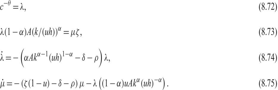
The interpretations of these first-order conditions are straightforward. Equation (8.72) suggests that on the margin, goods and services must be equally valuable in their two uses of consumption and investment, respectively. Equation (8.73) suggests that nonleisure time must be equally valuable in its two uses: production of goods and services and production of human capital. The differential equations (8.74) and (8.75) describe the evolution of the shadow prices of physical and human capital as a result of the accumulation of both types of capital.

From (8.72)–(8.75) and the accumulation equations (8.68) and (8.69), we can determine the endogenous variables. From (8.72) and (8.74), we can derive the familiar Euler equation for consumption:

From (8.73) and (8.75), it follows that

From the capital accumulation equation (8.68), the rate of growth of the per capita capital stock is given by

From the human capital accumulation equation (8.69), we have

Taking the logarithm of (8.73) and differentiating with respect to t, we get

Substituting (8.75), (8.77), (8.78), and (8.79) in (8.80), after some rearrangement, we get

On the balanced growth path, we have that

where g^* is the steady state endogenous growth rate.

From the steady state versions of (8.77) and (8.79), we can determine g^* and 1 − u^* as

alt=eq8-83-84.png>

The remaining endogenous variables on the balanced growth path, such as the ratio of physical to human capital and the ratio of aggregate consumption to the physical capital stock, can be determined by substituting in the steady state versions of (8.76) and (8.78).

From (8.83) and (8.84), the higher the productivity of human capital in the production of human capital, the higher the proportion of its nonleisure time that the household will devote to education and training. As a result, the endogenous growth rate is higher as well. In contrast, the higher the pure rate of time preference of households, the lower the endogenous growth rate and the proportion of its time that the household will devote to education and training, as opposed to the production of goods and services. This is because of higher discounting of the future, which makes education and training less attractive. Finally, a higher elasticity of intertemporal substitution in consumption results in a higher endogenous growth rate and a higher proportion of nonleisure time devoted to education and training.

In the special case where the elasticity of intertemporal substitution is equal to unity (θ = 1), the equations describing the determination of the endogenous growth rate and the time devoted to education and training simplify to

The time devoted to the accumulation of human capital is a positive function of productivity in the production function of human capital and a negative function of the discount factor of the representative household ρ − n.

To go beyond the analysis of the balanced growth path and describe the transitional dynamics of the model, we can define

From the definitions in (8.85), and (8.76), (8.78), (8.79), and (8.81), the transitional dynamics of the model are described by

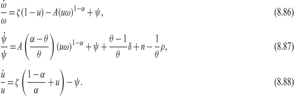
The system of the three differential equations (8.86), (8.87), and (8.88) determines the transitional dynamics of the three endogenous variables ω, ψ, and u.

In the steady state, we have

Thus, (8.86) – (8.89) determine the steady state endogenous variables ω, ψ, and u.

8.3