Dynamic Adjustment and the Balanced Growth Path
We can now move on to the question of how the balanced growth path is determined and the analysis of the dynamic adjustment of consumption, capital, and other real variables in the Ramsey model of the representative household.
The dynamic adjustment of the economy in the model is described by equations (4.20) for the accumulation of capital and (4.29) for the rate of growth of consumption. We have two first-order differential equations in two variables, k and c. We can use the two differential equations (4.20) and (4.29) to fully analyze the dynamic adjustment of the economy.
Equation (4.20) is given by

which describes the accumulation of capital per efficiency unit of labor.
Equation (4.29) can be modified to, assuming rt = Af′(k(t)) − δ,

which is the Euler equation for consumption per efficiency unit of labor. On the right-hand side of (4.29′), we have have used (4.22) to substitute for the real interest rate it terms of the marginal product of capital minus the depreciation rate of capital δ.
Once we determine the path of the capital stock and consumption, the paths of all other real variables (namely, output, the real interest rate, and the real wage) follow from the production function (4.15) and the marginal productivity conditions (4.22), which only depend on capital per effective unit of labor.
The solution of the second-order system of nonlinear differential equations (4.20) and (4.29′) can be described diagrammatically with the help of a phase diagram.
4.3.1 Dynamic Adjustment toward the Balanced Growth Path
The capital stock (per efficiency unit of labor) that ensures  (i.e., constant consumption per efficiency unit of labor) is determined by (4.29′) from the equalization of the marginal product of capital with the pure rate of time preference, plus the depreciation rate, plus the rate of technical progress g multiplied by θ.

Note that (4.40) implies that the steady state capital stock depends only on the parameters of the production function and four other parameters: the pure rate of time preference ρ, the depreciation rate δ, the inverse of the elasticity of intertemporal substitution in consumption θ, and the rate of technical progress g. Only technological and preference parameters affect the steady state per capita capital stock and, by means of the production function, the steady state per capita income. Note that the rate of growth of population n, unlike in the Solow model, does not affect steady state per capita capital and income.
Figure 4.1 depicts (4.40) as the vertical line  . We shall call it the steady state consumption locus, because along it, consumption per efficiency unit of labor is constant. This condition defines the steady state capital stock k*. If the capital stock is lower than k*, then the real interest rate is higher than ρ + θg, and from (4.29), consumption per efficiency unit of labor is rising. Hence the vertical arrows depicting rising consumption to the left of k* in figure 4.1. If the capital stock is higher than k*, then the real interest rate is lower than ρ + θg, and from (4.29), consumption per efficiency unit of labor is falling. Hence the vertical arrows depicting falling consumption to the right of k*.
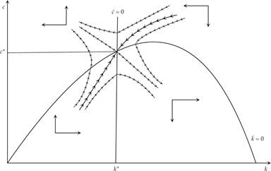
Figure 4.1 The balanced growth path and dynamic adjustment in the Ramsey model.
For  in (4.20), one can derive the relation between consumption and the capital stock (per efficiency unit of labor) that ensures a constant capital stock (per efficiency unit of labor).

which is depicted as the  curve in figure 4.1. Let us call it the steady state capital locus, because along it, the capital stock per efficiency unit of labor is constant. Because of the properties of the production function Af(k), it is upward sloping up to the point Af′(k) = n + g + δ, and downward sloping after that point. Thus, it achieves its maximum at the golden rule capital stock, for which the real interest rate is equal to the steady state growth rate n + g.
If consumption is higher than the level implied by (4.41), then savings are lower than the savings required to maintain a constant capital stock per efficiency unit of labor, and the capital stock per efficiency unit of labor is declining. Hence the left-pointing horizontal arrows above the constant capital curve in figure 4.1. If consumption is lower than the level implied by (4.41), then savings are higher than the savings required to maintain a constant capital stock per efficiency unit of labor, and the capital stock per efficiency unit of labor is increasing. Hence the right-pointing horizontal arrows above the constant capital curve in figure 4.1.
When (4.40) and (4.41) are satisfied simultaneously, the economy is on a balanced growth path, as both the capital stock and consumption per efficiency unit of labor are constant, which is equivalent to saying that per capita consumption and the per capita capital stock grow at the exogenous rate of technical progress g. The remaining real variables (such as output, the real wage, and the real interest rate) are also on a balanced growth path, because by the production function and the marginal productivity conditions, they depend solely on the capital stock per efficiency unit of labor.
The balanced growth path (or steady state equilibrium) at (k*, c*) is unique.
It is shown in figure 4.1, which depicts both (4.40) and (4.41) geometrically. Figure 4.1 also depicts the adjustment path leading to the steady state. In each section of figure 4.1, adjustment paths are determined by the direction of the resultant of the adjustment in consumption and capital. Thus, if both consumption and capital are rising in a section of the graph, then the economy moves toward the northeast. If both consumption and capital are falling in a section of the graph, then the economy moves toward the southwest. If consumption is rising and capital falling, the economy moves toward the northwest, and in the opposite case, toward the southeast. Both of these directions move the economy away from the steady state.The steady state (k*, c*) is called a saddle point: A unique adjustment path, the saddle path, leads to this saddle point, as the capital stock k is a predetermined (state) variable, and consumption c is a control variable. The saddle path goes through the northeast and the southwest parts of the diagram. For any initial value of k, consumption adjusts immediately to ensure that the economy is put on the unique saddle path leading to the steady state (the balanced growth path). All other adjustment paths, some of which are also depicted in figure 4.1, eventually diverge and lead the economy away from the balanced growth path, violating the transversality condition (4.33).
On the adjustment path, if the capital stock (per efficiency unit of labor) is lower that k*, consumption is also lower than c*, and the economy accumulates capital at a rate higher than n + g. During this process, capital and consumption per efficiency unit of labor are rising. The opposite happens if the initial capital stock (per efficiency unit of labor) is higher than k*. Then the capital stock and consumption per efficiency unit of labor are falling.
Consequently, the behavior of the economy on the adjustment path resembles in many ways the behavior of the economy in the Solow model.
There is convergence toward a unique long-run equilibrium (steady state or balanced growth path), regardless of initial conditions.The difference is that in the Ramsey model, savings behavior is not exogenous, but endogenous and optimal. At any point in time, the representative household chooses its consumption to maximize its intertemporal utility. Due to competitive markets, the optimal individual behavior of the representative household also maximizes social welfare. Both the short-run equilibrium (on the adjustment path) and the long-run equilibrium (on the balanced growth path) are not only Pareto efficient but also consistent with the maximization of social welfare.
It is worth looking into the properties of the steady state, or balanced growth path, in more detail. Although the capital stock, output, and consumption per efficiency unit of labor are constant, the per capita capital stock, output, and consumption increase continuously at rate g (the exogenous rate of technical progress). The real interest rate is fixed on the balanced growth path, as is the real wage per efficiency unit of labor. However, the real wage per employee w(t)h(t) grows at rate g, which causes a continuous increase in labor efficiency.
In the process of adjustment toward the balanced growth path from the left (i.e., when the initial capital stock per efficiency unit of labor is less than k*), per capita output and per capita consumption are rising faster than g, the real interest rate is on a downward path (because of the falling marginal product of capital), and the real wage per employee is rising faster than g (because of the rising marginal product of labor). The opposite happens in the process of adjustment to the balanced growth path from the right (i.e., when the initial capital stock per efficiency unit of labor is higher than k*).
4.3.2 The Balanced Growth Path and the Modified Golden Rule
The balanced growth path in the representative household model is similar to the balanced growth path in the Solow model.
The capital stock, output, and consumption per efficiency unit of labor are constant. Consequently, the savings ratio s = (y − c)/y is also constant on the balanced growth path. The aggregate capital stock, aggregate output, and total consumption are growing at the rate n + g. The per capita capital stock, per capita output, and per capita consumption are growing at the rate g.Consequently, most of the central predictions of the Solow model regarding the determinants of long-term growth are not dependent on the assumption of a constant exogenous savings rate. Even when the savings rate is endogenous, as in the Ramsey model, the exogenous rate of technical progress remains the sole determinant of the long-term growth rate of output, consumption, and real wages per capita.
The main difference between the Ramsey and Solow models regarding the balanced growth path is that in the Ramsey model, it is not possible for the capital stock on the balanced growth path to exceed the capital stock that corresponds to the golden rule. In the Solow model, with a sufficiently high savings rate, there may be dynamic inefficiency (i.e., the capital stock may end up higher than the one that corresponds to the golden rule). In such a case, it is possible to reduce the capital stock and increase consumption and social welfare. This possibility does not exist in the Ramsey model, because the optimization of intertemporal utility by the representative household rules it out.
In fact, in the representative household model, capital per efficiency unit of labor on the balanced growth path is always lower than the golden rule. This is because the representative household has a positive pure rate of time preference and discounts future utility. Thus, the representative household does not seek to maximize per capita consumption on the balanced growth path, as assumed in the derivation of the golden rule. Instead, it maximizes an intertemporal utility function that (given the positive pure rate of time preference) places a greater weight on current consumption relative to future consumption.
As can be seen from equation (4.40), which defines the steady state capital stock k*, or from figure 4.1, the steady state capital stock in the Ramsey model is lower than that corresponding to the golden rule, because the steady state real interest rate is equal to ρ + θg, which is higher than n + g. The steady state in the Ramsey model is often referred to as the modified golden rule.
Exercise 4.2 Assuming a Cobb-Douglas production function, derive the steady state of the representative household model from the system of differential equations (4.20) and (4.29). Discuss the determinants of all steady state variables. Also, analyze the stability of the system by linearizing the system around the steady state. Compare the steady state of the representative household model to the steady state corresponding to the golden rule. What determines the growth rate of per capita output, consumption, and real wages in the steady state?
4.3.3 Effects of a Permanent Increase in the Pure Rate of Time Preference
Figure 4.2 analyzes the impact of an increase in the pure rate of time preference of the representative household. It is assumed that the economy is initially on the balanced growth path (k*, c*) corresponding to the initial pure rate of time preference, and that at time t0, the pure rate of time preference increases permanently and unexpectedly.
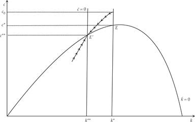
Figure 4.2 Short- and long-run effects of a permanent increase in the pure rate of time preference.
An increase in the pure rate of time preference rate leads to a shift of the steady state consumption line to the left. On the new balanced growth path (c**, k**), both consumption and capital will be lower. At time t0, consumption increases to c0 (because the capital stock is fixed) and puts the economy on the saddle path corresponding to the new balanced growth path. Because savings are lower than equilibrium investment, the economy begins to decumulate capital and gradually adjusts toward the new balanced growth path.
Figure 4.3 illustrates the impulse response function of consumption and capital per efficiency unit of labor after the increase in the pure rate of time preference. Consumption originally increases, which starts the process of gradual decumulation of capital per efficiency unit of labor, a gradual reduction in consumption, and a convergence to a new balanced growth path. This new balanced growth path is associated with lower capital and consumption compared to the previous path.
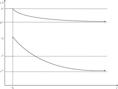
Figure 4.3 Impulse response function of consumption and capital stock following a permanent increase at t0 in the pure rate of time preference.
A decrease in the pure rate of time preference would have the opposite effects. On the new balanced growth path, both consumption and the capital stock will be higher. Consumption initially falls, the economy begins to accumulate capital, and there is gradual convergence toward the new balanced growth path with a higher capital stock and consumption per efficiency unit of labor.
The pure rate of time preference is a key determinant of savings behavior and steady state capital, output, and consumption in this model. The higher it is, the lower the inclination of the representative household will be to save for the future, and the lower the level of capital, output, and consumption will be on the balanced growth path.
4.3.4 Effects of a Permanent Increase in Total Factor Productivity
Figure 4.4 shows the impact of a permanent one-off increase in total factor productivity A. It is assumed that the economy is initially on the balanced growth path (k*, c*), corresponding to the initial total factor productivity, and that at time t0, total factor productivity increases permanently and unexpectedly.
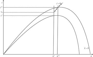
Figure 4.4 Short- and long-run effects of a permanent increase in total factor productivity.
An increase in total factor productivity leads to a shift of the steady state consumption locus to the right and to an upward shift in the locus of steady state capital. On the new balanced growth path (c**, k**), both consumption and capital will be higher. At time t0, consumption increases to c0 (because the capital stock is fixed) and puts the economy on the saddle path corresponding to the new balanced growth path. Because savings are higher than equilibrium investment, the economy begins to accumulate capital and gradually adjusts toward the new balanced growth path.
4.3.5 Effects of a Permanent Increase in the Rate of Growth of Population
As already shown by equation (4.40), on the balanced growth path, per capita capital and income are independent of the rate of growth of population. However, steady state consumption per capita depends negatively on the rate of growth of population, as can be seen from equation (4.41). A rise in the rate of growth of population calls for an increase in per capita savings to finance the higher steady state investment required to maintain a constant capital stock per efficiency unit of labor.
This result can also be shown diagramatically, with the help of figure 4.5. An increase in the population growth rate leads to a downward shift of the steady state capital locus but does not affect the steady state consumption locus ( ). On the new balanced growth path, only consumption will be lower. At time t0, consumption jumps immediately to c**. The capital stock is not affected, because savings increase immediately to match the higher equilibrium investment.
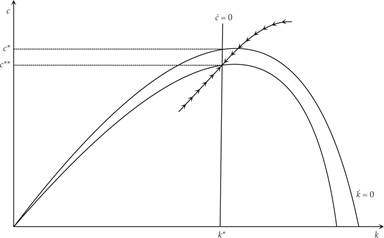
Figure 4.5 Effects of a permanent increase in the population growth rate.
Thus, because of the optimal savings behavior of the representative household, which internalizes the welfare of future generations, an increase in the population rate of growth does not affect per capita capital and income on the balanced growth path. This is because savings immediately match the extra equilibrium investment required as a result of the higher population growth. This behavior is a major difference between the Ramsey representative household model and the Solow model with an exogenous savings rate. As we shall see in chapter 5, it is also a major difference between the representative household and overlapping generations models as well.
4.4