The Ramsey Model of Economic Growth

As with the Solow model, in the Ramsey representative household model, we focus on the following set of endogenous variables: Y, aggregate output (or y, output per efficiency unit of labor); K, aggregate stock of (physical) capital (or k, capital per efficiency unit of labor); C, aggregate consumption (or c, consumption per efficiency unit of labor); r, real interest rate; and ŵ = wh real wage per worker (or w, real wage per efficiency unit of labor).

The exogenous variables and exogenous parameters in the model are defined as follows: t, time (a continuous exogenous variable); L, aggregate population and employment (an exogenous variable that depends on time); h, efficiency of labor (an exogenous variable that depends on time); n, rate of growth of population (exogenous parameter); g, rate of technical progress (exogenous parameter); δ, rate of depreciation of capital (exogenous parameter); and ρ, pure rate of time preference of households (exogenous parameter).

4.2.1 The Production Function

At each instant, the economy has a stock of capital, a given labor force, and given labor efficiency, which are combined to produce output. The production function has the form

This production function has all the properties of the neoclassical production function assumed in the Solow model. The marginal product of all inputs is positive but decreasing, there are constant returns to scale, and the Inada conditions are satisfied.⁵

As in the Solow model, let us assume that population growth and the efficiency of labor evolve according to

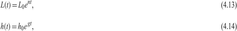
where L₀ and h₀ denote population and the efficiency of labor at time 0.

Due to the assumption of constant returns to scale, the production function can be expressed in intensive form (i.e., per efficiency unit of labor) as

where y = Y/hL is output per efficiency unit of labor, k = K/hL is capital per efficiency unit of labor, and f(k) = F(k, 1) is the production function per efficiency unit of labor.

4.2.2 The Utility Function of the Representative Household

All households in this economy are assumed to be identical. Thus, we shall eventually focus our attention on the behavior of only one of them: the representative household. Households are indexed by j, where j is uniformly distributed between zero and 1. Thus, j ∈ [0, 1].

The utility function of household j depends on the level of its per capita consumption. The household is assumed to have an infinite time horizon and to maximize the intertemporal utility function⁶

where c_j(t) denotes the per capita consumption of household j at instant t; u is the instantaneous utility function of household j; and ρ is the pure rate of time preference of household j, an exogenous preference parameter. The number of members of the household is given by L_j(t) and is the same for all households. Thus, it follows that the relation between the members of individual households j and total population is given by

We assume that the instantaneous utility function of the household takes the form

where θ > 0, and ρ−n− (1 −θ)g > 0. This functional form is the constant elasticity of intertemporal substitution utility function already introduced in chapter 2 and in subsection 4.2.1, with 1/θ being the elasticity of intertemporal substitution of consumption.

The assumption that ρ − n − (1 − θ)g > 0 is sufficient to ensure that the intertemporal utility function (4.16) is well defined and converges to a finite value. This assumption is also sufficient to ensure that the economy eventually converges to a steady state, or balanced growth path.

As already mentioned, as θ tends to unity, one can prove, using l’Hopital’s rule, that the utility function tends to the logarithmic utility function. That is, in the case θ = 1, we have

Because all households are the same, we shall henceforth drop the subscript j and concentrate not on average household consumption, but on consumption per efficiency unit of labor. If c_j(t) is the average consumption per member of household j, and all households are the same, then it follows that

where ĉ(t) is per capita consumption at instant t.

Then consumption per efficiency unit of labor c(t) is defined by

Substituting equation (4.18) into equation (4.17) and the resulting equation in equation (4.16), and then taking into account that h(t) and L(t) increase at exogenous rates g and n, respectively, we arrive at an intertemporal utility function of the representative household, expressed in terms of consumption per efficiency unit of labor:

where , and β = ρ − n − (1 − θ)g > 0.

The representative household thus maximizes (4.19), which is equivalent to (4.16), subject to the constraint that its savings result in the accumulation of real assets, which take the form of physical capital.

4.2.3 The Accumulation of Capital and the Optimality of the Decentralized Competitive Equilibrium

As in the Solow model, the accumulation of capital per efficiency unit of labor in the economy is determined by

Equation (4.20) shows that the change in aggregate physical capital per efficiency unit of labor is determined by the difference of two terms: current investment (savings) per efficiency unit of labor minus equilibrium investment (i.e., the investment required to maintain capital per efficiency unit of labor at its current level).

A social planner who seeks to maximize the intertemporal utility of the representative household (4.19), subject to the constraint (4.20), would thus determine the savings behavior that maximizes social welfare. The question is whether (4.20) is also the budget constraint facing the representative household itself in a decentralized competitive equilibrium. If so, the optimal savings behavior of the representative household would also maximize social welfare, and the decentralized equilibrium would be socially optimal. To answer this question, one needs to consider the budget constraint facing the representative household in a decentralized competitive economy.

Assume a competitive economy, in which each member of the representative household provides a unit of labor, and savings take the form of investment in physical capital. The real wage per worker equals the real wage per efficiency unit of labor w(t) times the efficiency of labor h(t). Consequently, the per capita labor income of the household at time t equals

where w(t) is the real wage per efficiency unit of labor.

Households rent their capital stock to competitive firms in a competitive capital market. The per capita income from capital of the representative household is given by

where r(t) + δ is the rental price of capital in the competitive capital market.

Consequently, in a decentralized competitive economy, the accumulation of capital per efficiency unit of labor is determined by the savings of the representative household, and is given by

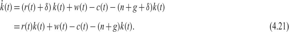
The representative household takes the evolution of w(t) and r(t) + δ as given, as these are determined in competitive labor and capital markets. In such markets, capital and labor are paid their respective marginal product. Thus,

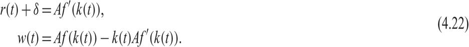
Substituting the pair of equations (4.22) into (4.21), we end up with (4.20). Hence, the budget constraint faced by the representative household, in the form of the asset accumulation equation (4.21), is the same as the budget constraint (4.20) faced by the economy as a whole and by the hypothetical social planner.

In this model, due to the assumption of competitive markets, maximizing the intertemporal utility function of a representative household is essentially under the same constraint as the one that would be used by a social planner (i.e., the economywide budget constraint (4.20)). The problem of the representative household is the same as that of a hypothetical omnipotent social planner.

Consequently, the competitive equilibrium in the model of the representative household is fully optimal. A decentralized competitive equilibrium in which each household maximizes its own utility function over time, under its private budget constraint, would lead to the same outcome as that of an omnipotent social planner who had as her objective the maximization of the intertemporal utility function of the representative household, under the appropriate aggregate budget constraint.

In the case of the representative household model with full and competitive markets, we have an application of the first theorem of welfare economics: When markets are competitive and complete, and there are no externalities, the decentralized equilibrium is optimal, because it maximizes social welfare.

4.2.4 Conditions for Utility Maximization by the Representative Household

To find the first-order conditions for the maximization of (4.19) under the accumulation equation (4.21), we define the current value Hamilton function as

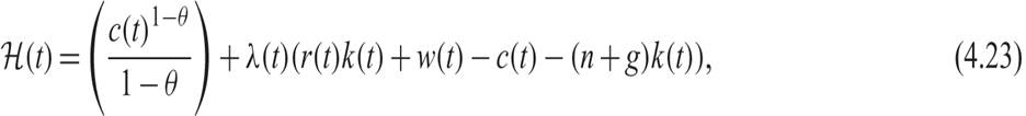
where λ(t) is the multiplier of the Hamilton function; λ(t) can be interpreted as the “shadow price” of the marginal instantaneous change of the capital stock at t (marginal investment).

The Hamilton function is thus defined as the sum of the instantaneous utility of consumption plus the value of the change in the capital stock, priced at the shadow price λ(t). An optimal plan must maximize the Hamilton function at each instant t, provided that the shadow value is chosen correctly. From the maximum principle, the first-order conditions for the maximization of the Hamilton function coincide with the first-order conditions for the maximization of (4.19), subject to the sequence of the accumulation equations (4.21).

The first-order conditions for the maximization of the Hamilton function are

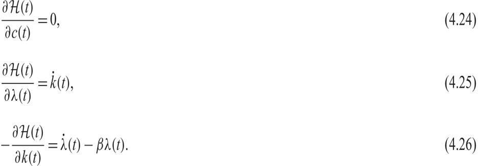
Here (4.24) implies

and (4.26) implies

Finally, (4.25) implies the capital accumulation equation (4.21).

Equation (4.27) suggests that consumption must be chosen at each instant so that its marginal utility is equal to the shadow price of the marginal unit of savings invested in capital. At each instant, goods must be equally valuable at the margin, either as consumption or as investment.

Equation (4.28) implies that capital gains (i.e., the rate of change of the shadow price of capital λ(t)) must be equal to the difference between the discount factor of the household β and the rate of return of capital per efficiency unit of labor r(t) − n − g. This condition essentially ensures that the total rate of return of a marginal unit of capital, including capital gains, is equal to the discount factor of the household β.

This interpretation can be confirmed by rearranging (4.28) as

It is straightforward to show that if a social planner maximized the intertemporal utility function of the representative household, subject to the economywide capital accumulation condition (4.20), then the relevant first- order conditions would be (4.27) and

By the definition of the real interest rate in (4.21), (4.28) is exactly the same as the equation above, which confirms that the competitive equilibrium maximizes social welfare in this model.

4.2.5 The Euler Equation for Consumption

We can examine the first-order conditions by eliminating λ(t) between (4.27) and (4.28). Taking the first derivative of (4.27) with respect to time, after using (4.28) and the definition of β, we end up with the following differential equation for c:

which is the Euler equation for consumption per efficiency unit of labor. The growth rate of consumption per capita is positive if the real interest rate exceeds the pure rate of time preference of the representative household. In addition, the higher the elasticity of intertemporal substitution of consumption is, the higher the growth rate of consumption will be for a given difference between the real interest rate and the pure rate of time preference of the representative household. In equation (4.29), g has a negative impact because c is consumption per efficiency unit of labor, and its denominator increases at a rate g (the exogenous rate of technical progress). This is why g must be subtracted.

If (4.29) is rewritten in terms of per capita consumption, we would have

where ĉ is per capita consumption. This equation is the same as (4.11) and has the same interpretation.

In what follows, we concentrate on the Euler equation for consumption per efficiency unit of labor (4.29). If the economy is on a balanced growth path, consumption per head will be growing at the exogenous rate of technical progress g, and consumption per efficiency unit of labor will be constant. Thus, from (4.29), the real interest rate on the balanced growth path will be equal to ρ + θg. As we shall see below, there is a unique constant real interest rate that is consistent with a balanced growth path in this model.

4.2.6 The Intertemporal Budget Constraint of the Representative Household

Equation (4.29) determines the rate of change of consumption on the optimal path. To determine the level of consumption on the optimal path, one must solve the two differential equations (4.29) and (4.21), which determine the optimal path of consumption and capital accumulation of the representative household.

Let us first solve the capital accumulation equation of the representative household (4.21). This is a first-order linear differential equation with variable coefficients. As a result, its solution for any T ≥ 0 takes the form⁷

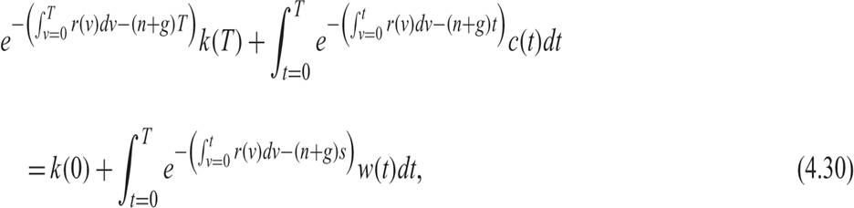
which describes the intertemporal budget constraint of the representative household with horizon T. This intertemporal budget constraint implies that at time 0, the present value of labor income between time 0 and time T, plus the initial capital stock at time 0, must be equal to the present value of consumption between time 0 and time T, plus the present value of the capital stock at time T. The term that includes the integral of interest rates is a term that converts one unit of income, consumption, or capital at time t to its present value at time 0. If the real interest rate is fixed at r, then the term would simplify to − rt.

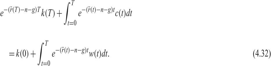
We can define the average real interest rate between time 0 and time t as

With this definition of the average real interest rate, (4.30) can be written as

If the horizon of the household were T, then the optimal capital stock at instant T would be equal to zero. If the capital stock at T were positive, then the household could increase its utility by consuming the rest of its capital just before T, and hence the path would not be optimal. Thus, a positive capital stock at T would not be optimal. If the capital stock at T were negative, then the household would be accumulating unsustainable debts (negative capital) along the optimal path, which would be violating its intertemporal budget constraint. We should therefore assume that on the optimal path, k(T) = 0. A similar assumption was made in the two-period model of chapter 2, when we assumed that the household consumes its remaining capital in period 2.

This type of condition is called a transversality condition, and it ensures that the present value of consumption of the household cannot exceed or fall short of its total wealth. Total wealth consists of the initial capital stock of the household plus the present value of its labor income. Thus, because we must have that k(T) = 0, for a finite time horizon T, the intertemporal budget constraint of the representative household takes the form

Taking into account the transversality condition, the intertemporal budget constraint implies that at time 0, the present value of labor income between time 0 and time T, plus the initial capital stock at time 0, must be equal to the present value of consumption between time 0 and time T. The question that arises is: What is the transversality condition when the horizon of the household is infinite, as we have assumed?

4.2.7 The Transversality Condition with an Infinite Time Horizon

If the time horizon of the household is infinite, as we have been assuming, then we should take the limit of (4.32) as T tends to infinity. In this case, the first term on the left in (4.32) should tend to zero. That is, we should have

If this condition is not satisfied (for example, if the above limit is positive), then the household could increase its intertemporal utility along the optimal path by consuming a larger part of its capital. If the above limit is negative, then the household would be accumulating unsustainable debts (negative capital) along the optimal path, which is not consistent with its intertemporal budget constraint. Therefore, the only optimal path consistent with the intertemporal budget constraint of the representative household is the one that satisfies (4.33), which requires that the present value of its capital stock tends to zero as time tends to infinity.

Condition (4.33) is the infinite-horizon transversality condition. It is satisfied as long as the capital stock per efficiency unit of labor does not increase (or decrease) at a rate faster than r − n − g, which is the same as saying that the aggregate capital stock does not increase (or decrease) at a rate faster than r.

As already mentioned (and is proved explicitly in section 4.3), the real interest rate on the balanced growth path is equal to ρ + θg. As a result, if the economy is on the balanced growth path, the transversality condition takes the form

given that u′(c(T)) > 0. Equation (4.34) is the transversality condition on the balanced growth path.

Given that the transversality condition (4.33) must be satisfied, the intertemporal budget constraint of a representative household with an infinite time horizon takes the form

which implies that the present value of consumption of a representative household with an infinite time horizon equals its total wealth, defined as its initial capital stock (physical capital) plus the present value of current and future labor income (human capital).

4.2.8 The Consumption Function of the Representative Household with an Infinite Horizon

If we solve (integrate) the differential equation describing the Euler equation for consumption (4.29), then we find that consumption at time t is defined by

Substituting (4.36) in the intertemporal budget constraint (4.35) and solving for c(0) yields

where

is the present value of labor income, and

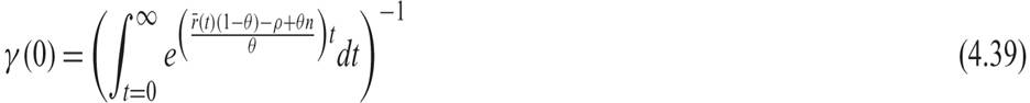
is the proportion of total wealth consumed in period 0.

Equation (4.37), along with definitions (4.38) and (4.39), determines the level of consumption for the representative household. Consumption at time 0 is a proportion γ(0) of total wealth. (4.37) allows us to deduce the properties of the consumption function of the representative household.

The representative household consumes a share of its total wealth equal to γ(0). This share depends on the evolution of the average future real interest rates, the pure rate of time preference rate ρ, the elasticity of intertemporal substitution of consumption 1/θ, and the population growth rate n.

The impact of the average real interest rate on the proportion of total wealth that is consumed depends on the elasticity of intertemporal substitution of consumption 1/θ. An increase in average real interest rates has two kinds of effects on the average consumption to total wealth ratio: an intertemporal substitution effect and an income effect. The intertemporal substitution effect induces the household to substitute current for future consumption, as it increases the cost of current consumption relative to future consumption. This tends to decrease current consumption. The income effect of an increase in real interest rates increases income from capital and tends to increase both current and future consumption. This tends to increase current consumption.

If the elasticity of intertemporal substitution of consumption is greater than one (i.e., θ < 1), then consumption as a proportion of total wealth decreases when real interest rates rise and savings increase, because the negative intertemporal substitution effect is stronger than the positive income effect. In such a case, the intertemporal substitution effect prevails. If the elasticity of intertemporal substitution is less than unity (θ > 1), then consumption as a proportion of total wealth increases when interest rates rise, because the positive income effect is stronger than the negative intertemporal substitution effect. Finally, if θ = 1, which is the case with logarithmic preferences, the two results cancel each other out, and consumption as a proportion of total wealth is independent of the path of real interest rates. These effects are exactly the same as in the two-period model analyzed in chapter 2.

It is worth deriving the consumption function when the real interest rate is fixed at r, as happens in the steady state. In this case, (4.39) takes the form

For γ(0) to be positive, we must have that r < (ρ − θn)/(1 − θ). On the balanced growth path, the real interest rate is constant and equal to r = ρ + θg. As a result, on the balanced growth path, the share of total wealth that is consumed is equal to

From the assumptions we have made to ensure a well-defined intertemporal optimization problem for the representative household (see equation (4.19)), this share is positive.

In the case where θ = 1 (i.e., logarithmic preferences), from (4.39), the share of consumption to total wealth is given by

Given that we have assumed that ρ > n, with a unitary elasticity of intertemporal substitution of consumption, the share of consumption in total wealth is equal to the difference between the pure rate of time preference and the population growth rate.

Finally, it is important to note that the overall impact of real interest rates on consumption is not limited to the impact on the propensity to consume out of total wealth. An increase in real interest rates leads to a decrease in the present value of future labor income, reducing the overall wealth of the representative household and leading to a reduction in consumption, even if the elasticity of intertemporal substitution is equal to one. Essentially, the effects of real interest rates on the present value of income from employment (i.e., the wealth effects of real interest rates) reinforce the negative substitution effect on current consumption.

4.3