The Optimal Intertemporal Path of Consumption

To introduce the problem of the optimal intertemporal choice of consumption, in chapter 2 we assumed a household that lives only for two periods and maximizes an intertemporal utility function that depends on the level of consumption in each of the two periods.

We now extend the two-period analysis to the problem of a household with a long time horizon equal to T. This is the problem posed and solved by Ramsey [1928]. We assume that time is continuous and that the representative household has a finite time horizon equal to T.

The household supplies a unit of labor per instant and has a exogenous flow of labor income equal to w. It can borrow and lend freely in the capital market at a real interest rate r. The household has an initial endowment of an interest yielding asset equal to a(0). It is assumed to maximize the following intertemporal utility function:

subject to

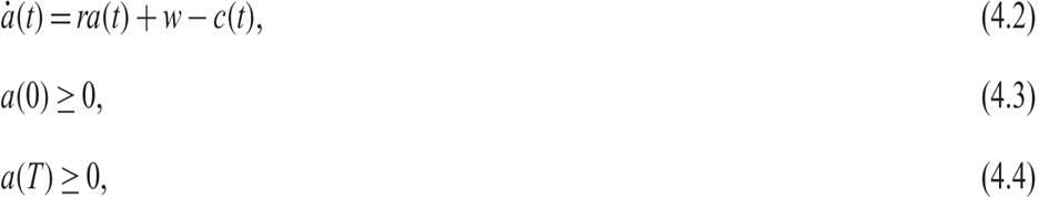
where u is the instantaneous utility function of the household, which depends on consumption of goods and services (u is twice differentiable and concave); and ρ is the pure rate of time preference, the rate at which the household discounts future utilities. (4.2) is the asset accumulation equation, (4.3) defines the initial assets of the household, and (4.4) is a terminal condition that ensures that the household respects its intertemporal budget constraint. The household cannot end up with negative assets at the end of its horizon T. A condition such as (4.4) is called a transversality condition.

From the maximum principle, the first-order conditions for the maximization of (4.1), subject to the accumulation constraint (4.2), are the same as the first-order conditions for the maximization of the current-value Hamilton function, or “Hamiltonian”, which for this problem is defined by³

where λ(t) is the current value multiplier of the asset accumulation constraint; λ(t) can be interpreted as the shadow price of the marginal instantaneous change of household assets at time t.

The Hamilton function is thus defined as the sum of the instantaneous utility of consumption plus the value of the change in the assets of the household, priced at the shadow price λ(t). An optimal plan must maximize the Hamilton function at each instant t, provided that the shadow value is chosen correctly. The first-order conditions for the maximization of the Hamilton function coincide with the first-order conditions for the maximization of (4.1), subject to the sequence of the accumulation equations (4.2).

The first-order conditions for the maximization of the current-value Hamilton function are given by

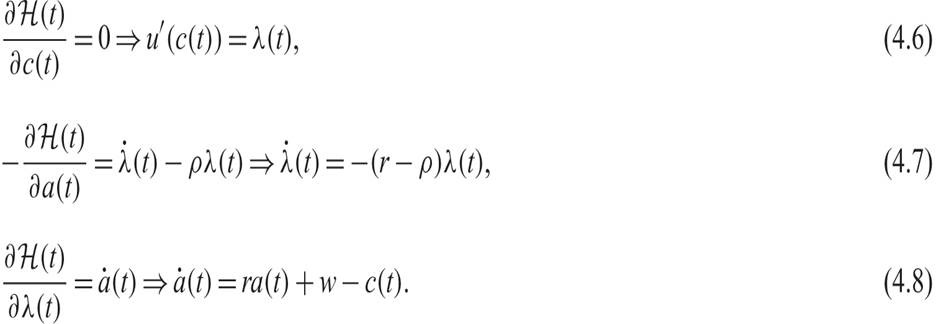
From (4.6), on the optimal path, we see that the multiplier λ(t) (which is the value of the marginal increase in assets) is equal to the marginal utility of consumption. Thus, the household is indifferent between one extra unit of consumption and one extra unit of savings. Equation (4.7) shows that on the optimal path, the real interest rate plus the expected marginal increase in the value of assets (capital gain) is equal to the pure rate of time preference of the household. Finally, (4.8) is the asset accumulation equation.

We can use the first-order conditions (4.6) and (4.7) to characterize the behavior of consumption along the optimal path.

Substituting (4.6) and (4.9) into (4.7) results in

which is the Euler equation for consumption. It is nothing more than the expression in continuous time of the typical condition for optimality: The marginal rate of intertemporal substitution of consumption is equal to the marginal rate of intertemporal transformation of current to future consumption. The interpretation of (4.10) is analogous to that of the Euler equation for the two-period problem already analyzed in chapter 2.⁴

Because the second derivative of the instantaneous utility function is assumed to be negative (i.e., the marginal utility is declining with consumption), the change in consumption will have the same sign as the difference between the real interest rate and the pure rate of time preference. If the real interest rate is higher than the pure rate of time preference, then consumption will be continuously increasing. In the opposite case, consumption will be continuously decreasing. If the real interest rate is equal to the pure rate of time preference, then consumption will be constant on the optimal path.

If we assume that the instantaneous utility function of the household has the form of (2.39), with a constant elasticity of intertemporal substitution of consumption 1/θ, then (4.10) takes the form

which implies that the optimal consumption of the household increases, remains constant, or decreases, depending on whether the real interest rate exceeds, equals, or falls short of the pure rate of time preference, respectively.

Exercise 4.1 Derive equation (4.11) from an intertemporal optimization problem of a representative household with a CEIS utility function.

This optimality rule is logical. The higher the real interest rate is relative to the pure rate of time preference, the greater will be the incentive for the representative household to reduce current consumption and invest in assets with a rate of return r (and so enjoy higher future consumption). So if the real interest rate is higher than the pure rate of time preference, consumption per capita will be growing along the optimal path. If the real interest rate is lower than the pure rate of time preference, consumption per capita will be declining along the optimal path. Finally, if the real interest rate is equal to the pure rate of time preference, consumption will be constant along the optimal path. In this last case, there will be full consumption smoothing.

Equation (4.11) also highlights the role of the elasticity of intertemporal substitution 1/θ. The higher the elasticity of intertemporal substitution is, the easier it will be for the household, in utility terms, to substitute consumption over time (and thus the easier it is to substitute current for future consumption). Consequently, for a given difference between the real interest rate and the pure rate of time preference, the growth rate of per capita consumption is higher, the higher the elasticity of intertemporal substitution. We can now proceed to incorporate the optimal consumption behavior of a representative household in a full-blown growth model.

4.2