The Natural Rate of Unemployment and Aggregate Demand Policies

The instability of the Phillips curve led Milton Friedman to define the concept of the natural rate of unemployment. According to Friedman [1968], a market economy tends to converge toward an equilibrium unemployment rate u₀, which can be labeled as the natural rate of unemployment.

Friedman [1968] argued that trying to reduce the unemployment rate below the natural rate, by increasing aggregate demand and inflation, would only meet with temporary success. As inflationary expectations adjust to the higher inflation, unemployment will tend to return to its natural rate. One would need continuous increases in aggregate demand and inflation to keep unemployment below its natural rate. If at some point, the government stopped increasing aggregate demand and inflation, then the unemployment rate would return to its natural rate, and the economy would be saddled with high inflation.

Friedman thus argued against the use of discretion in the determination of aggregate demand policies and in favor of fixed rules for monetary and fiscal policy that would deliver low and steady inflation. In the fullness of time, this proved to be a devastating argument against discretionary policies of the Tinbergen-Theil variety.²²

To analyze the argument, assume that the Phillips curve is linear and given by

where a and b are positive constant parameters.

According to the definition of the natural rate of unemployment, the economy is at its natural rate when inflationary expectations are equal to actual inflation. Consequently, the natural rate of unemployment in this simple model is determined by

The natural rate of unemployment is thus constant, as a and b are assumed to be constant parameters.²³

When analyzing aggregate demand policies in a context in which inflation is determined by the Phillips curve (15.39), a key question that has to be answered is: How are inflationary expectations formed?

15.5.1 The Path of Inflation and Unemployment under Adaptive Expectations

For many years, the dominant approach to the formation of expectations in macroeconomics was the adaptive expectations hypothesis.

Consequently, the adjustment of inflationary expectations according to this hypothesis would take the form

where 0 ≤ λ < 1. According to (15.41), in each period, inflationary expectations are adjusted by a percentage 1 − λ of the divergence between actual and expected inflation in the previous period.

It is assumed that λ is less than one, because if it is equal to one, then there is no adjustment in expectations, and we have the assumption of nonadaptive or static expectations.

What are the properties of this specific hypothesis for the adjustment of expectations? From (15.41), we have

Inflationary expectations under the adaptive expectations hypothesis are a geometric distributed lag of past inflation rates. Thus, adaptive expectations are backward looking.

Given that λ < 1, from the difference equation (15.42), if inflation were to be held constant at an equilibrium rate π_A, inflationary expectations would gradually converge to that equilibrium inflation rate π_A. The speed of adjustment is equal to 1 − λ. The smaller is λ, the speedier will be the adjustment of inflationary expectations to actual equilibrium inflation. In the extreme case where λ = 0, expectations converge after one period. At the other extreme (in the case where λ = 1), expectations never converge, and we essentially have nonadaptive or static expectations.

Substituting (15.42) in the Phillips curve (15.39) and solving for unemployment, one gets

If inflation were held constant at any inflation rate (say, π_A), unemployment would gradually converge to its natural rate u₀ with a speed of adjustment equal to 1 − λ (that is, the speed of adjustment of inflationary expectations).

What would happen in the case where the government did not have a fixed target for inflation, but a socially desirable fixed target for unemployment u_A, which happened to be lower than the natural rate of unemployment u₀? In this case, the government and the monetary authorities would presumably use discretionary aggregate demand policies to maintain unemployment below its natural rate u₀ at u_A, where u_A < u₀.

From the unemployment equation (15.43), if the government aimed to keep unemployment constant at u_A < u₀, inflation would evolve according to

The difference equation (15.44) has a unit root, and thus inflation does not converge. In fact, it increases from period to period by a percentage that depends on the difference between the natural rate of unemployment rate u₀ and the government’s target unemployment rate u_A. As the government uses discretionary aggregate demand policies to keep unemployment below its natural rate, it will be causing a constant increase in inflation, so that inflation is always higher than the rising adaptive inflationary expectations. Otherwise, unemployment cannot be maintained below its natural rate.²⁵

This case is depicted in figure 15.10. When the government and the monetary authorities seek to maintain unemployment below its natural rate u₀ at the lower rate u_A, inflation and inflationary expectations start increasing. To keep unemployment below its natural rate, actual inflation must be higher than expected inflation. Under adaptive expectations, this can only happen if inflation increases continuously. If the government and the monetary authorities allow the unemployment rate to return to its natural rate, then inflation will stop increasing.²⁶

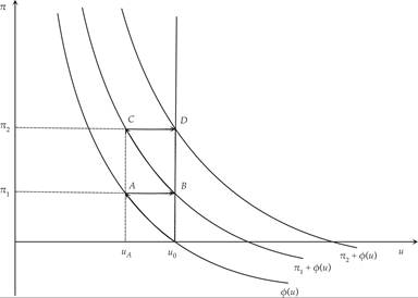
Figure 15.10 Continuous shifts of the Phillips curve due to rising inflationary expectations.

Let us now assume, as in the case of the AD-AS model, that the government and the monetary authorities are not concerned only about inflation or only about unemployment, but about both. They use aggregate demand policies to minimize a quadratic loss function that depends on both inflation and unemployment. Assume that this function takes the form²⁷

where ζ is the relative weight that the government attaches to deviations of inflation relative to unemployment from their socially desirable levels π_A and u_A, respectively. The objective function (15.45) is minimized subject to the Phillips curve (15.39), with the government taking inflationary expectations as given.

From the first-order conditions for a minimum of (15.45), subject to the Phillips curve (15.39), we get

Under the optimal discretionary aggregate demand policy, the marginal welfare cost of deviations of unemployment from the government target equals the marginal welfare cost of deviations of inflation from target. If both targets could be achieved, (15.46) would be automatically satisfied, but if the government cannot achieve both targets simultaneously, optimal second-best policy must satisfy (15.46).

Using the unemployment equation (15.43) to substitute for unemployment in (15.46), we end up with the following equation for inflation under the optimal policy:

Substituting (15.47) in the first-order condition (15.46), unemployment under the optimal policy follows

From (15.47) and (15.48), inflation and unemployment gradually converge to steady state values equal to

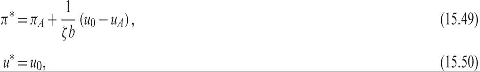
where π^* and u^* denote steady state inflation and unemployment, respectively.

Equations (15.49) and (15.50) suggest that if the government is using discretionary aggregate demand policies to pursue an unemployment target that is lower than the natural rate of unemployment, but it also cares about inflation (ζ > 0), both inflation and unemployment converge to unique steady state values. However, steady state inflation turns out to be higher than the socially desirable inflation target π_A, and steady state unemployment is also higher than the socially desirable unemployment target u_A and is equal to the natural rate u₀.²⁸

Note from (15.49) that the discrepancy between steady state inflation and the socially desirable inflation target π_A is larger,

• the larger the discrepancy is between the natural rate of unemployment and the socially desirable unemployment target u_A,

• the smaller is the weight ζ of inflation relative to unemployment in the social loss function (15.45), and finally,

• the smaller is the impact of unemployment on inflation in the Phillips curve (15.39).

These parameters reflect the incentives of the government to reduce unemployment and create unanticipated inflation under a discretionary aggregate demand policy.

In the attempt to reduce unemployment below the natural rate, the government drives actual inflation and inflationary expectations above the socially desirable inflation target to a level that balances (1) the marginal welfare cost of deviations of unemployment from the government target with (2) the marginal welfare cost of deviations of inflation from the government target. Note that (15.49) and (15.50) satisfy the first-order condition for the minimization of the social loss function (15.45). Thus, at the steady state inflation rate (15.49), inflation is so high that the government has no further incentive to use discretionary aggregate demand policies to reduce unemployment below its natural rate, because this would bring about a further increase in the already high inflation rate.

We have thus demonstrated that the use of discretionary aggregate demand policies to pursue an unemployment target that is lower than the natural rate does not affect steady state unemployment. This ends up at the natural rate u₀ anyway. But it does affect steady state inflation, which turns out to be higher than the socially desirable government target.

15.5.2 Rules versus Discretion in Aggregate Demand Policy

Because steady state unemployment is equal to the natural rate u₀ anyway, a better policy outcome would be for inflation to be equal to π_A, the socially optimal inflation rate, rather than to the higher π^*.

The inflationary bias of discretionary aggregate demand policies arises because policymakers cannot commit to the low, socially desirable inflation π_A: Under discretion, when inflationary expectations are equal to π_A, they have the incentive to create surprise inflation to reduce unemployment. For this reason, under discretion, the economy ends up with both higher inflation and higher unemployment than what is socially desirable.

Suppose that instead of having the discretion to choose aggregate demand policies in every period to minimize (15.45), the government is committed to using aggregate demand policies to keep inflation constantly at the socially optimal rate π_A. Thus for all periods, we have

Then steady state inflation is also equal to π_A, and steady state unemployment is equal to u₀. The inflationary bias of discretionary aggregate demand policies disappears, as the government is committed to following the rule (15.51). Then it cannot succumb to the temptation to use aggregate demand policies to reduce unemployment and thus create unanticipated inflation. Thus, under commitment to the policy rule (15.51), the economy would end up with unemployment at the natural rate, which is higher than what is socially desirable (but is the same as under the discretionary policy), and inflation that is equal to the socially desirable level π_A and not higher. The inflationary bias disappears, and the policy outcome is better than the policy outcome under discretion.

A graphical illustration of this argument can be seen with the help of figure 15.11. Assume that originally, the economy is at the natural rate of unemployment, with zero inflation (point 0). The government decides to expand aggregate demand to reduce unemployment. This has the effect of increasing inflation along the original Phillips curve. The economy ends up at point 1, where the original Phillips curve is tangent to the highest possible social indifference curve between inflation and unemployment. Point 1 implies lower unemployment and higher inflation. In the short run, the government is better off, as the welfare loss associated with point 1 is lower than that associated with point 0. Note that point A, which implies the lowest-possible welfare loss, cannot be attained. But point 1 is not a stable equilibrium, because inflationary expectations start adapting to the higher inflation π₁, and the Phillips curve starts shifting upward.

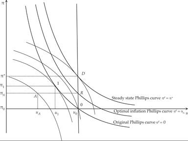
Figure 15.11 Determination of steady state inflation and unemployment under discretion and commitment to an inflation rule.

Thus, the government will need to further increase aggregate demand to keep unemployment below the natural rate. This will generate a further increase in inflation, further upward revisions of inflationary expectations, and so on.

The process will only stop when the economy ends up at point D (D for “discretion”), and expectations adapt to the inflation rate π^*. At point D, the government no longer has an incentive to further expand aggregate demand to reduce unemployment. The welfare costs from further increases in inflation exceed the welfare benefits from the reduction in unemployment. Thus, D is a stable steady state equilibrium.

Under commitment to a inflation rule that keeps inflation equal to π_A, the economy converges to the steady state equilibrium R (R for “rules”). Point R is preferable to D, because it is associated with lower steady state inflation (π_A < π^*) and the same unemployment rate. The problem is that at R, the government has a short-run incentive to renege on its commitment and expand aggregate demand to reduce unemployment. The short-run marginal welfare gain from the reduction in unemployment is higher than the short-run marginal welfare loss from the rise in inflation. Thus, the commitment mechanism must be binding for the government not to succumb to the temptation of increasing aggregate demand.

These results were first demonstrated by Kydland and Prescott [1977], under the assumption of rational expectations. As we have demonstrated in this section, they hold in the steady state under adaptive expectations too. The discretionary (time-consistent) policy is not intertemporally optimal, in the sense that there is a better policy outcome under commitment to the rule (15.51). However, the rule (15.51) is not time-consistent, because the government has an incentive to deviate from it in every period to minimize (15.45). Thus, the intertemporally optimal steady state policy rule is time inconsistent: It is not optimal in the short run.

This case is an important example of the time inconsistency of optimal policy in dynamic settings, in which policymakers have objectives that conflict with the objectives of private agents (Kydland and Prescott [1977]). The time-consistent policy is not optimal, and the optimal policy is time inconsistent. Thus, binding commitment mechanisms are required to ensure that an optimal policy rule, such as (15.51), is implemented in every period.

15.5.3 Inflation and Unemployment under Rational Expectations

Our analysis so far has been based on the assumption of adaptive expectations. One of the consequences of the realization that the original Phillips curve is unstable was the adoption of the hypothesis of rational expectations. The hypothesis of rational expectations gradually became the key hypothesis regarding the formation of expectations, not only about inflation, but also about all future variables that affect the behavior of households and firms, as well as governments.²⁹

In this particular context, rational expectations implies that households and firms form inflationary expectations that take into account the incentives of governments to use discretionary policies to choose between inflation and unemployment. It is thus worth analyzing the implications of the rational expectations hypothesis for this model of the natural rate.

From the first-order conditions for a minimum of the social loss function (15.45), subject to the Phillips curve (15.39), we get that under discretionary policies, equation (15.46) must necessarily hold. Using the Phillips curve (15.39) to substitute for unemployment in (15.46), we get

Because there are no stochastic disturbances, the hypothesis of rational expectations implies that expected and actual inflation will coincide. Thus, (15.52), combined with the rational expectations hypothesis, implies that

Under rational expectations, in the absence of stochastic disturbances, inflation is always equal to expected inflation. Thus, inflation jumps to steady state inflation immediately. Consequently, unemployment also jumps to its natural rate immediately. Discretionary aggregate demand policies cannot affect unemployment even in the short run, and they only result in both short-run and steady state inflationary bias, because of the incentives of the government to create surprise inflation and the immediate adjustment of expectations to anticipate these incentives.

In contrast, under commitment to the time-inconsistent policy rule (15.51), inflation is equal to

The unemployment rate is equal to the natural rate u₀ in all periods.

Thus, under rational expectations, the dynamic adjustment to the steady state is immediate, because there are no other sources of persistence in this model. The suboptimality of discretionary policy is even starker in this case, and the argument in favor of commitment to rules such as (15.51) is even stronger.³⁰

15.6