The Phillips Curve and Inflationary Expectations

We have already demonstrated that the main difference between the original Keynesian models and the corresponding classical models is the assumption of nominal rigidity in both prices and wages, or (in the case of the AD-AS model) only nominal wages.

15.4.1 The Phillips Curve and the Trade-off between Inflation and Unemployment

Since the late 1950s, a central point of reference for Keynesian models has been the Phillips curve, a negative relationship between unemployment and inflation identified and estimated econometrically by Phillips [1958]. The Phillips curve was combined with the IS-LM model of aggregate demand to simultaneously determine both inflation and unemployment. Thus, the Phillips curve essentially replaced the aggregate supply curve of the AD-AS model, which was based on fixed nominal wages, and helped determine both unemployment and inflation.

The curve that Phillips estimated econometrically for the United Kingdom took the form

where φ(u₀) = 0 and φ′(u) < 0. In equation (15.37), π denotes inflation, u is the unemployment rate, and u₀ is the zero inflation unemployment rate. The function φ relating inflation and unemployment estimated by Phillips is nonlinear. Its shape is depicted in figure 15.7.¹⁹

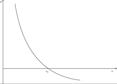
Figure 15.7 The Phillips curve.

In the context of the basic Keynesian model, combining the IS-LM model of the determination of aggregate demand with the Phillips curve, one could deduce that an increase in aggregate demand would lead to higher real output and employment, lower unemployment, and a rise in inflation along the Phillips curve. Conversely, a decline in aggregate demand would lead to a lower level of real output and employment, higher unemployment, and a reduction of inflation along the Phillips curve.

Inspired by Phillips [1958] Samuelson and Solow [1960] estimated a Phillips curve between price inflation and unemployment for the United States. These authors argued that the short-term problem of macroeconomic policy could be seen as the determination of the level of aggregate demand in order to select the socially desirable combination of inflation and unemployment on the Phillips curve. In times of recession, an increase in aggregate demand will lead to a reduction in unemployment, but at the cost of higher inflation. In times of economic boom and high inflation, inflation could be reduced through a reduction in aggregate demand, but this would result in higher unemployment.

The Samuelson-Solow argument can be understood with the help of figure 15.8, which depicts the Phillips curve and the indifference map of policymakers between inflation and unemployment. Because both inflation and unemployment are assumed to be undesirable, the indifference curves are concave to the origin. The closer an indifference curve is to the origin, the higher will be the implied social welfare. Samuelson and Solow argued that because the Phillips curve implies a negative relationship between inflation and unemployment, it acts as a constraint on the options of policymakers. The latter will maximize social welfare at point E in the figure, where the Phillips curve is tangent to the highest-possible indifference curve. Point E is thus associated with the optimal feasible combination of inflation and unemployment under a discretionary macroeconomic policy.²⁰

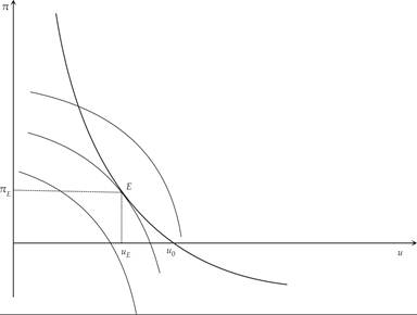
Figure 15.8 The Phillips curve and the socially optimal combination of inflation and unemployment.

Note that at point E, both inflation and unemployment are positive, and policymakers would prefer lower inflation and unemployment. However, an equilibrium with both lower inflation and lower unemployment is not feasible, as the only feasible combinations lie on the Phillips curve, which acts as constraint for macroeconomic policy.

15.4.2 Instability of the Phillips Curve and Inflationary Expectations

Since the mid-1960s, the negative relationship between inflation and unemployment began to shift. Higher inflation led to a reduction of unemployment only temporarily, because unemployment rose after a while to return to its original level without a reduction in inflation. This puzzle was finally attributed to shifts in inflationary expectations.

As argued by Phelps [1967] and Friedman [1968], a sustained increase in inflation would lead to expectations of higher future inflation on the part of households and firms. The result of this would be that inflation would have to increase even further to achieve a reduction in unemployment. Essentially, Phelps and Friedman argued that the Phillips curve has the form

where φ(u₀) = π − π^e = 0 and φ′(u) < 0, and π^e is expected inflation.

A shift of the Phillips curve (15.38) due to an increase in inflationary expectations is shown in figure 15.9. Assume that initially, inflation and inflationary expectations are equal to zero and unemployment is at u₀. The government and the monetary authorities choose to increase aggregate demand to reduce unemployment, and the economy moves to point A, where unemployment has fallen, but inflation has increased. As inflationary expectations gradually adjust to the higher inflation, the Phillips curve moves up, and thus, the economy moves gradually toward point C. Inflation rises above π_A at the unemployment rate u_A. Point A is no longer feasible. If the government and the monetary authorities want to maximize social welfare, they have to adjust monetary and fiscal policy to move the economy to point B, which implies higher inflation and unemployment relative to A. This would again be temporary, because it would lead to a further gradual upward adjustment in inflationary expectations, a further shift in the Phillips curve, and a further increase in inflation and unemployment.

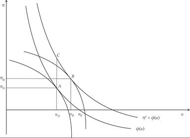
Figure 15.9 Shifts of the Phillips curve due to inflationary expectations.

15.5