Dynamic Simulations of a Calibrated Solow Model

To further investigate the process of dynamic adjustment that characterizes the Solow model, we can simulate, for specific numerical values of the parameters, the transition from a balanced growth path to another path when there is an exogenous permanent change in particular parameters (such as the savings rate, total factor productivity, or the rate of growth of population).

To simulate the model numerically, let us convert it from a continuous-time model to a discrete-time model.

3.8.1 The Solow Model in Discrete Time

Instead of assuming that time is a continuous variable, time is now measured as successive discrete time periods, where t = 0, 1, 2, …. The variable x_t indicates the variable x in period t.

Population and the efficiency of labor grow at constant exogenous rates n and g per period, respectively. Thus, we have

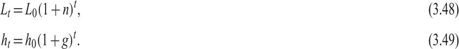
The production function is given by

and is characterized by constant returns to scale and diminishing returns of individual factors.

As in the case of continuous time, we assume that the consumption function is characterized by a fixed savings rate s:

The accumulation of capital is determined by

Thus, in discrete time, the accumulation of capital per efficiency unit of labor is given by

It can easily be shown diagrammatically (see figure 3.8) that the difference equation (3.53) converges to a unique equilibrium.

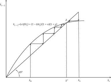
Figure 3.8 Convergence in the Solow model in discrete time.

In figure 3.8, the curve depicts the accumulation equation (3.53), and the 45° straight line the steady state equilibrium condition k_t = k_t+1) = k^*. The process of convergence is determined by (3.53), and the equilibrium toward which the economy converges determines the balanced growth path.¹⁵

3.8.2 The Calibrated Solow Model

For the purposes of simulation, let us use a calibrated version of the model, assuming that the production function is Cobb-Douglas:

where A > 0 is total factor productivity, and 0 < α < 1 is the exponent (share) of capital in the production function. 1 − α is the exponent of labor.

Substituting (3.54) in (3.53), the capital accumulation equation is given by

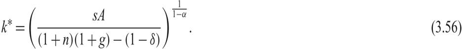
From (3.55), the steady state capital stock, per efficiency unit of labor, is given by

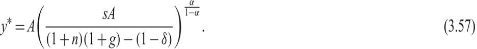
The remaining variables are all functions of k, and their steady state values are functions of k^*. Output is given by (3.54), and steady state output is given by

Consumption is given by

Finally, the real interest rate and the real wage are given by

Simulating (3.55) numerically, for specific parameter values, we can calculate the dynamic adjustment of capital toward the balanced growth path.

3.8.3 Dynamic Simulations of the Model

The calibrated model relies on the following values of the initial parameters: A = 1, α = 0.333, s = 0.30, n = 0.01, g = 0.02, and δ = 0.03. These are the same as the values used to calculate the speed of convergence in section 3.5.

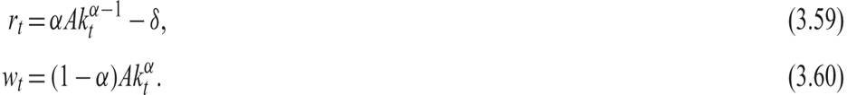
Figure 3.9 shows the impulse response functions of the calibrated Solow model following a permanent increase in the savings rate s of 1%. In the simulation shown, the economy is on the initial balanced growth path, and after period 1, the savings rate increases permanently and unexpectedly by 1%, from 0.30 (i.e., 30%) to 0.303 (30.3%). The increase in the savings rate leads to a decrease in consumption, a gradual accumulation of capital, a gradual increase in production, a gradual increase in real wages and a gradual fall in real interest rates. The reason for increasing real wages is the gradual increase in the marginal product of labor caused by the accumulation of capital. The reason for the gradual reduction in the real interest rate is the gradual reduction of the marginal product of capital caused by the accumulation of capital. The economy gradually converges toward a new balanced growth path. In this new balanced growth path, capital per efficiency unit of labor is higher by approximately 1.5%, output and real wages by 0.5%, consumption by 0.07% (due to the increase in the savings rate), and the real interest rate has fallen by 0.07 percentage points.

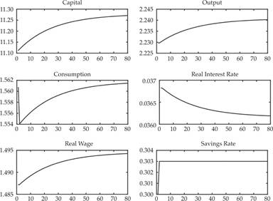
Figure 3.9 Impulse response functions of the Solow model following a permanent increase in the savings rate of 1%.

Figure 3.10 presents the impulse response functions of the model following an increase in total factor productivity A of 1%. In this simulation, the economy is on the initial balanced growth path, and after period 1, total factor productivity A increases permanently and unexpectedly by 1%, from 1 to 1.01.

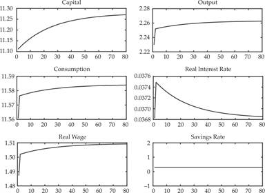
Figure 3.10 Impulse response functions of the Solow model following a permanent increase in total factor productivity of 1%.

Finally, figure 3.11 shows the impulse response functions of the model following an increase in the rate of population growth n by 1%. In this simulation, the economy is on the initial balanced growth path, and after period 1, the rate of growth of population n increases permanently and unexpectedly by 1%, from 1% to 1.01%. This increase leads to a gradual decumulation of capital and a gradual decline in output, consumption, and the real wage (the marginal product of labor). The real interest rate (marginal product of capital) gradually increases. The economy gradually converges to a new balanced growth path. On this path, capital per efficiency unit of labor is lower by about 0.25%; output, consumption, and real wages are lower by 0.08%; and the real interest rate has increased from 3.68% to 3.69%. The negative effects of an increase in population growth on steady state per capita income and consumption in the Solow model are not insignificant, but neither are they huge.

Figure 3.11 Impulse response functions of the Solow model following a permanent increase in the rate of population growth of 1%.

3.9