Convergence with a Cobb-Douglas Production Function
The Solow model with a Cobb-Douglas production function can be solved analytically not only for the steady state variables, as we have done so far, but also for their evolution during the process of convergence.
This is because the first-order differential equation that characterizes the convergence process in this case has the form of a Bernoulli equation, which can be converted to a linear differential equation in the capital-output ratio, and thus solved analytically.With a Cobb-Douglas production function, output per efficiency unit of labor is given by

Therefore, the adjustment of capital per efficiency unit of labor is given by

This is a Bernoulli equation, which can be converted to a linear differential equation if we define a new variable z:14

This variable is none other than the capital-output ratio. From (3.42), it follows that

By substituting (3.41) into (3.43) we get
alt=eq3-44.png>
where λ = (1 − α)(n + g + δ). The parameter λ is just the speed of convergence. (3.44) is a first-order linear differential equation in the variable z (the capital output ratio) and can be solved as

Substituting from the definition of the capital-output ratio with a Cobb-Douglas production function, the convergence process of capital and output per efficiency unit of labor is given by
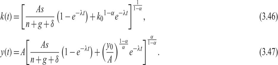
As time tends toward infinity, the limit of (3.46) and (3.47) is the balanced growth path, as determined by (3.35) and (3.36).
3.8