The Process of Economic Growth and the Solow Model
The Solow model, like any other economic model, is based on relatively simple and, many would claim, largely unrealistic assumptions. However, it constitutes a significant improvement on previous models, which did not rely on the neoclassical production function.
Such were, for example, the models of Harrod [1939] and Domar [1946], which were based on Leontieff [1941] production functions with constant coefficients and a zero elasticity of substitution between capital and labor.The question is whether the model of Solow (and all models based on similar assumptions about the technology of production) can offer an adequate and satisfactory account of the actual process of economic growth. To answer this question, we must delve a little deeper into the main empirical facts about long-run growth.
3.6.1 The Kaldor Stylized Facts of Economic Growth
An important early codification of the main empirical features pertaining to long run growth, is due to Kaldor [1961], who based them on the long-run growth experience of Great Britain and the United States. According to Kaldor, a growth theory should be consistent with the following six stylized facts about long-run growth:
1. Per capita GDP is growing over time, and the growth rate is not declining.10
2. Physical capital per worker is growing over time.
3. The long run-rate of return on capital is roughly constant.
4. The long-run capital-output ratio is roughly constant.
5. The shares of labor and capital in GDP do not display a long-term trend.
6. The growth rate of labor productivity varies substantially across countries.
These stylized facts continue to be accepted today, with the addition of some newer ones.11
At a general level, the Solow model is roughly consistent with all the above stylized empirical characteristics. However, the process of physical capital accumulation, which is the main engine of economic growth in the Solow model, is not sufficient as an explanation of either the long-run growth of output per worker that has been observed historically in almost all developed economies of the world or the large differences in output per worker between developed and less developed economies.
Only a small part of these phenomena can be explained by the accumulation of physical capital. The largest part appears to be due to technical progress and to differences in total factor productivity and the efficiency of labor, which are considered exogenous in the Solow model.12
3.6.2 Differences in Per Capita Output and Income between Developed and Less Developed Economies
The Solow model identifies three sources of differences in per capita income and output per worker between countries or between periods: first, differences in capital per worker; second, differences in total factor productivity and labor efficiency; and third, differences in initial conditions.
To simplify the analysis of the impact of each of these differences, let us use the Solow model and assume a Cobb-Douglas production function.
In the Solow model based on the Cobb-Douglas production function, capital per efficiency unit of labor on the balanced growth path is defined by the condition

From (3.34), it follows that the steady state capital stock per efficiency unit of labor is given by
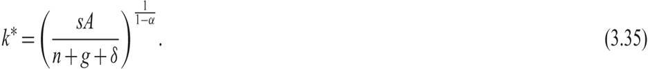
From (3.35) and the production function (3.4), output per efficiency unit of labor is given by
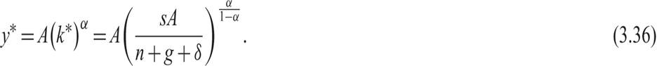
The per capita product on the balanced growth path is thus given by

where a hat over a variable denotes the per capita magnitude.
Based on (3.37), differences in capital per worker, for realistic estimates of the parameters of the model, cannot explain the differences in output per worker that we observe in the real world. For example, let us assume that we want to explain a ratio x in output per worker between two economies, economy 1 (a developed economy) and economy 2 (a less developed economy).
From (3.37), assuming that all other parameters except for the capital stock are the same between the two economies, we must have that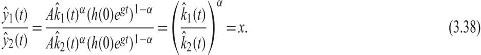
To explain this ratio, capital per worker should differ by x to the power 1/α, where α is the share of capital in domestic income. Since α is of the order of 1/3, to explain why GDP per worker in developed countries is currently 20 times higher than in less developed countries, capital per worker should be 8,000 times (20 raised to the third power) higher. But this is not the case. In developed economies, capital per worker is only 20–30 times higher than in less developed economies. Thus, we cannot account for differences in per capita output and income solely on the basis of differences in the per capita capital stock.
We can certify this indirectly as well. If the differences in output per worker were due only to differences in physical capital per worker, then we should observe huge differences in the rate of return to capital between periods and between countries. However, such huge differences in the rate of return to capital do not exist.
To explain the large differences between developed and less developed countries on the balanced growth path, we should allow for other differences, such as disparities in total factor productivity and the efficiency of labor. Allowing for such differences in (3.38), we have that
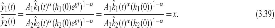
Differences in total factor productivity and the initial efficiency of labor, along with those in physical capital per worker, can explain almost all differences in output per worker that we observe in the real world. For example, if the developed countries have capital per worker 30 times higher than the less developed countries have, a total factor productivity that is three times that of the less developed countries (A1 = 3A2), and three times the initial efficiency of labor (h1(0) = 3h2(0)), then (3.39) predicts that, along the balanced growth path, their output per worker and their per capita income will be about 20 times higher than those of the less developed countries.
However, total factor productivity and the efficiency of labor are not explained by the Solow model but are instead considered as exogenous. Therefore, one could say that this model does not explain the process of long-run growth; it only assumes such growth.13
This is why this model, like all models based on similar assumptions about the technology of production and technical progress, is often referred to as an exogenous growth model. It assumes that total factor productivity A, the initial efficiency of labor h(0), and the rate of technical progress g are all exogenous parameters.
3.6.3 Conditional Convergence
Our analysis in subsection 3.6.2 makes it clear that the process of convergence predicted by the Solow model does not entail convergence to the same per capita income for all economies. The per capita income to which an economy converges is determined by (3.36) and (3.37) to be
If parameters such as the rate of savings and investment s, total factor productivity A, the population growth rate n, the depreciation rate δ, and the initial efficiency of labor h(0) differ between two economies, these economies will converge toward different levels of per capita income, even if along the balanced growth path, per capita income is growing at the same rate of technological progress g.
Convergence toward different levels of per capita income, which depend on the parameters characterizing the structure of different economies, is called conditional convergence. The per capita income toward which economies converge in the Solow model (and in the other exogenous growth models that we shall analyze in the next few chapters) depends on their specific structural characteristics. Not all economies converge to the same per capita income. Each economy converges to the per capita income determined by its own technological, demographic, and savings (investment) parameters.
3.7