Effects of Monetary Growth in an OLG Model
We next turn to the analysis of the impact of the growth rate of the money supply in the OLG model of Blanchard and Weil.
We assume, as in the Blanchard-Weil model of chapter 5, that the economy consists of overlapping generations of households born at different times in the past.
Each generation has an infinite time horizon. At each instant t, nL(t) households are born, where L(t) is total population at time t, and n is the growth rate of the number of households and the overall population. Each household has one member and provides one unit of labor. Consequently, the growth rate of the labor force is also n. Unlike the representative household model, OLG models do not internalize the welfare of future generations. We now assume that the instantaneous utility function of households depends on both consumption and real money balances, because of the liquidity services of holding money.7.4.1 The Blanchard-Weil Model with Money
The household born at time j chooses a path for consumption and real money balances to maximize the intertemporal utility function

subject to the instantaneous asset accumulation equation

and the transversality condition
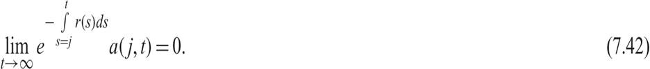
The variables and parameters are defined as in the case of the representative household model: ρ is the pure rate of time preference of households, and u is a quasi-concave instantaneous utility function; c(j, s) denotes the consumption of the household born at time j at time s; m(j, s) is real money balance of the household born at time j at time s; a(j, s) denotes average assets of the household born at time j at time s; w(s) denotes the real wage per efficiency unit of labor at time t, assumed to the same for all households; h(s) denotes labor efficiency per worker; τ(s) denotes average taxes (minus transfers) per household at time s; r(s) is the real interest rate at time s; and π(s) is inflation, which is equal to expected inflation.
Assuming that the instantaneous utility function u takes the form of (7.4) with an intertemporal elasticity of substitution equal to unity (as in chapter 5), we can write the instantaneous utility function as5

From the first-order conditions for a maximum and assuming that the assets of households consist of physical capital, government bonds, and money, we can derive the aggregate money demand function, the equation describing the evolution of aggregate consumption, and the equation describing capital accumulation:6
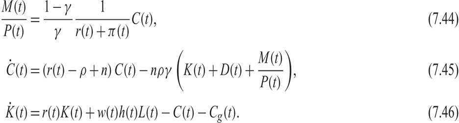
Expressing (7.44), (7.45), and (7.46) per efficiency unit of labor and assuming that the government has a constant target for primary government expenditure and government debt per efficiency unit of labor (as well as a constant target for the rate of growth of the money supply), we get
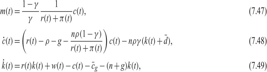
where in (7.48), we have used (7.47) to substitute for the stock of real money balances per efficiency unit of labor.  is government debt per efficiency unit of labor, assumed constant.
Using the marginal productivity conditions to replace the real interest rate and the real wage per efficiency unit of labor, (7.48) and (7.49) can be written as
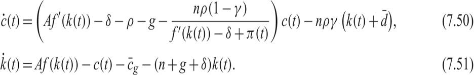
Equations (7.50) and (7.51) can be used to analyze both the balanced growth path and the adjustment path in terms of the exogenous parameters of the model and the policy variables describing government expenditure, government debt, and the growth rate of the money supply.
7.4.2 Real Effects of the Growth Rate of the Money Supply
From (7.50) and (7.51), we have on the balanced growth path


Equations (7.52) and (7.53) jointly determine real private consumption and real capital per efficiency unit of labor on the balanced growth path as a function of parameters of technology, household preferences, the population growth rate, and the rate of exogenous technical progress, as well as the parameters describing fiscal and monetary policy.
The balanced growth path and the relevant unique saddle path are shown graphically in figure 7.2. In the figure,  is the steady state consumption function (7.52), and
  is the steady state capital accumulation function (7.53). The balanced growth path and the adjustment path have the usual properties that characterize the model of Blanchard and Weil. The balanced growth path is a saddle point. The new element here is the impact of the growth rate of the money supply on private consumption.7
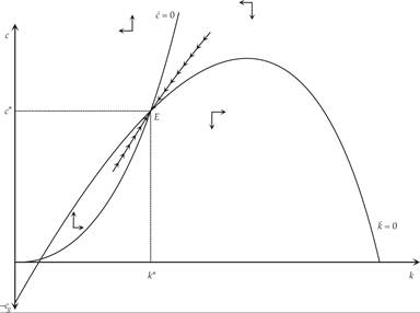
Figure 7.2 The balanced growth path and the adjustment path in the Blanchard-Weil model with money.
A permanent increase in the growth rate of the money supply μ leads to a permanent increase in inflation and nominal interest rates. This in turn leads to a reduction in the demand for real money balances. In this model, the decline in real money balances leads to a corresponding reduction in private consumption by current generations, thus increasing aggregate savings and causing the accumulation of physical capital.
The relevant analysis is shown in figure 7.3. A previously unanticipated permanent increase in the rate of growth of the money supply, which leads to an increase in inflation, results in a heavier inflation tax for the current generations. These generations hold higher real money balances compared to future generations, who do not hold real money balances. This causes a reduction in their current consumption, an increase in aggregate savings, and the initiation of a process of accumulation of physical capital. At the time of the implementation of the policy, consumption falls from cE to c0. The economy adjusts toward a new balanced growth path E′, which implies higher capital, output, and consumption per efficiency unit of labor, due to the substitution toward physical capital caused by higher inflation. In this model, the superneutrality of money does not apply, because the inflation tax impacts different generations differently, and the redistribution it causes in favor of future generations reduces current consumption and increases savings by current generations.
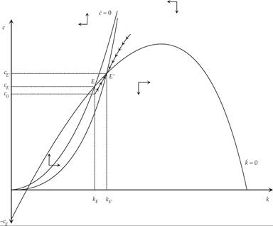
Figure 7.3 Dynamic effects of an increase in the growth rate of money supply in the Blanchard-Weil model with money.
Thus, as with Ricardian equivalence, the superneutrality of money does not apply in an OLG model like that of Blanchard and Weil model, because in this model current generations do not internalize the welfare of future generations.
7.4.3 A Dynamic Simulation of the Effects of a Rise in the Growth Rate of the Money Supply in a Calibrated Blanchard-Weil Model
To gain some insights into the quantitative impact of the growth rate of the money supply in the OLG model of Blanchard-Weil, let us examine simulations of the model for specific parameter values, assuming the usual Cobb-Douglas production function of the form

Consequently, the model being simulated consists of discrete time versions of (7.50) for the evolution of private consumption, (7.51) for the accumulation of capital, (7.54) for the production function, (7.47) for the money demand function, the marginal productivity conditions (7.20) and (7.21) for the real interest rate and real wages, the Fisher equation (7.5) for the nominal interest rate, and (7.14) for inflation.
Where the marginal product of capital or labor appears, this is derived from the production function (7.54).The simulations use the usual parameter values, as in chapters 3–6. For γ, the share of consumption in the utility function, we use a value equal to 97.5%. With regard to the parameters of fiscal policy it is assumed, as in chapter 6, that,  = 0.5 and
  = 0.5. Thus, the paramerer values used are A = 1, α = 0.333, ρ = 0.02, n = 0.01, g = 0.02, δ = 0.03, γ = 0.975,
  = 0.5, = 0.5.
Figure 7.4 shows the dynamic effects of a permanent change in the growth rate of the money supply from 5% to 10% in the calibrated Blanchard-Weil model. In the simulation, this change is accompanied by corresponding reductions in taxes, which are continuously equal to the increase in the inflation tax on real money balances. There is thus no impact on primary government expenditure or government debt.
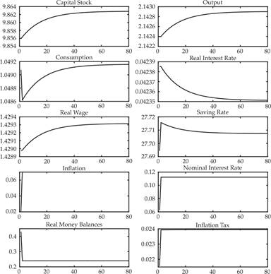
Figure 7.4 Dynamic simulation of an increase in the growth rate of money supply in a calibrated Blanchard-Weil model with money.
The change in the growth rate of the money supply from 5% to 10% reduces private consumption expenditure immediately, due to the reduction in the real money balances of current generations. This causes an increase in savings and initiates a process of capital accumulation that leads the economy toward a new balanced growth path with a higher capital stock, higher output, higher private consumption, and higher real wages per efficiency unit of labor. In contrast, the real interest rate falls.
Inflation rises by five percentage points, the same as the rise in the rate of growth of the money supply, and roughly the same happens to nominal interest rates.However, note that the impact of a change in the growth rate of the money supply on the real economy is extremely small. A doubling of the rate of growth of the money supply from 5% to 10% leads to an increase in steady state real per capita income (and real wages) of only 0.02%, and a reduction in the real interest rate by only 0.005 percentage points (i.e., from 4.239% to 4.234%). The overall savings rate in the balanced growth path rises from 27.69% to 27.70%, again a very slight increase. In contrast, inflation rises by five percentage points (from 2% to 7%), and nominal interest rates rise from 6.24% to 11.24%. The rise in the nominal interest rate is due to the rise in inflation, because the fall in the real interest rate is negligible. The rise in nominal interest rates results in a fall of the demand for real money balances by 44.5%. This is the only significant real effect of the doubling of the rate of growth of the money supply. All other real effects are miniscule.
We see therefore that, as with deviations from Ricardian equivalence, deviations from the superneutrality of money in OLG models (such as the Blanchard-Weil model) are quantitatively limited. The changes are small, because these deviations depend on the product of two quantitatively small parameters: the rate of growth of population (which determines the rate of entry of new generations in the economy) and the pure rate of time preference of households (which determines the percentage of total household wealth that is consumed). With the assumptions made, for a population growth rate of 1% per year and a pure rate of time preference of 2%, their product is equal to just 0.02%.
7.5