Exercises
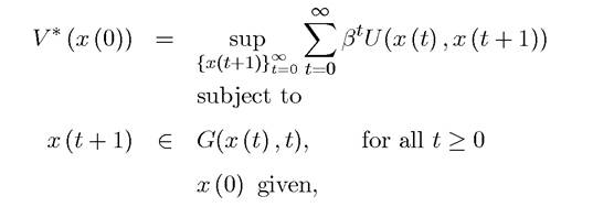
EXERCISE 6.1. Consider the formulation of the discrete time optimal growth model as in Example 6.1. Show that with this formulation and Assumptions 1 and 2 from Chapter 2, the discrete time optimal growth model satisfies Assumptions 6.1-6.5.
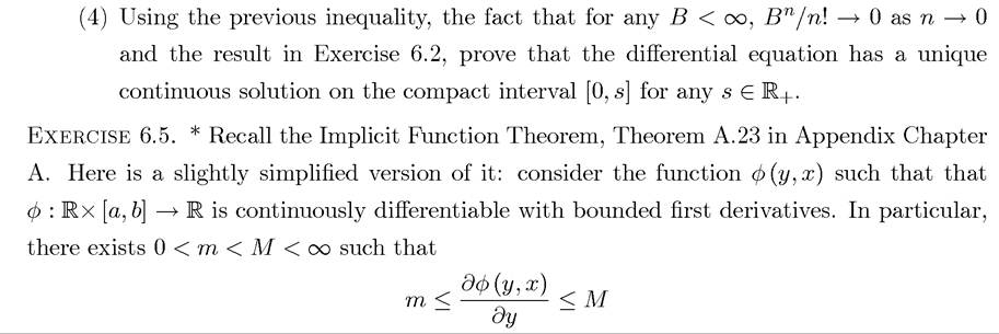
Exercise 6.2. * Prove that if for some n ∈ Z+ Tn is a contraction over a complete metric space (S, d), then T has a unique fixed point in S.
Exercise 6.3. * Suppose that T is a contraction over the metric space (S, d) with modulus β ∈ (0,1). Prove that for any z,z0 ∈ S and n ∈ Z+, we have

Discuss how this result can be useful in numerical computations.
Exercise 6.4. *
(1) Prove the claims made in Example 6.3 and that the differential equation in (6.7) has a unique continuous solution.
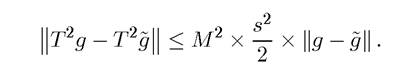
(2) Recall equation (6.8) from Example 6.3. Now apply the same argument to Tg and Tg and prove that
(3) Applying this argument recursively, prove that for any n ∈ Z+, we have 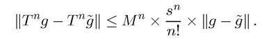
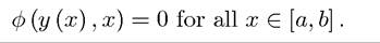
for all x and y. Then the Implicit Function Theorem states that there exists a continuously differentiable function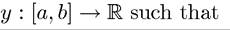
Provide a proof for this theorem using the Contraction Mapping Theorem, Theorem 6.7 along the following lines:
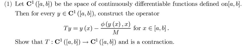
(2) Applying Theorem 6.7 derive the Implicit Function Theorem.
Exercise 6.6. * Prove that T defined in (6.15) is a contraction.
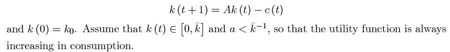
Exercise 6.7. Let us return to Example 6.4.
(1) Prove that the law of motion of capital stock given by 6.28 monotonically converges to a unique steady state value of k* starting with any ko > 0. What happens to the level of consumption along the transition path?
(2) Now suppose that instead of (6.28), you hypothesize that 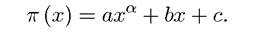
Verify that the same steps will lead to the conclusion that b = c = 0 and a = βa.
(3) Now let us characterize the explicit solution by guessing and verifying the form of the value function. In particular, make the following guess: V (x) = A lnx, and using this together with the first-order conditions derive the explicit form solution.
Exercise 6.8. Consider the following discrete time optimal growth model with full deprecisubject to
ation:
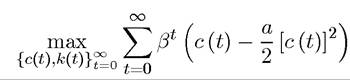
(1) Formulate this maximization problem as a dynamic programming problem.
(2) Argue without solving this problem that there will exist a unique value function V (k) and a unique policy rule c = π (k) determining the level of consumption as a function of the level of capital stock.
(3) Solve explicitly for V (k) and π (k) [Hint: guess the form of the value function V (k), and use this together with the Bellman and Euler equations; verify that this guess satisfies these equations, and argue that this must be the unique solution].
Exercise 6.9. Consider Problem Al or A2 with x ∈ X ⊂ R and suppose that Assumptions 6.1-6.3 and 6.5 hold. Prove that the optimal policy function y = π (x) is nondecreasing if
Exercise 6.10.
Show that in Theorem 6.10, a sequence that satisfies the Euler
 equations, but not the transversality condition could yield a suboptimal plan.
Exercise 6.11. Consider the following modified version of Problem A1:
where the main difference from Problem A1 is that the constraint correspondence is timevarying. Suppose that for all t, that
 is continuously differen
tiable, concave and strictly increasing an its first K arguments, and that the correspondence  is continuous and convex-valued. Show that a sequence
 with
with
 , is an optimal solution to this problem given x (0), if it satisfies (6.21) and (6.25).
Exercise 6.12. Let us return to the problem discussed in Example 6.5.
(1) Show that even when the sequence of labor earnings is not constant over
time, the result in Exercise 6.11 can be applied to obtain exactly the same result as in Example 6.5. In particular, show that the optimal consumption profile is still given by (6.31).
(2) Using the transversality condition together with a (0) and find an expres
sion implicitly determining the initial level of consumption, c (0). What happens to this level of consumption when a (0) increases?
(3) Consider the special case where u (c) = ln c.
Provide a closed-form solution for c (0).(4) Next, returning to the general utility function u (∙), consider a change in the earnings

What is the effect of this on the initial consumption level and the consumption path?
Provide a detailed economic intuition for this result.
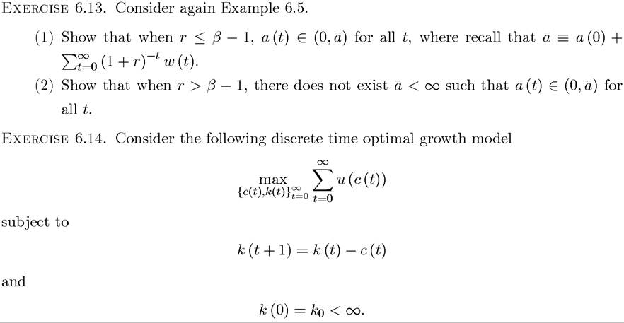
Assume that u (∙) is a strictly increasing, strictly concave and bounded function. Prove that there exists no optimal solution to this problem. Explain why.
Exercise 6.15. Consider the following discrete time optimal growth model with full depreciation:
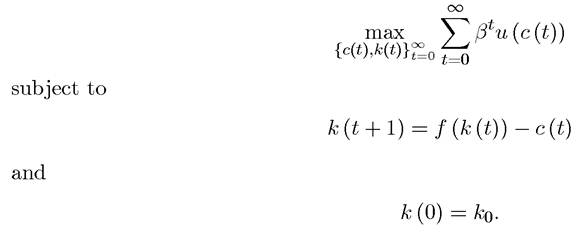
Assume that u (∙) is strictly concave and increasing, and f (∙) is concave and increasing.
(1) Formulate this maximization problem as a dynamic programming problem.
(2) Prove that there exists unique value function V (k) and a unique policy rule c = π (k), and that V (k) is continuous and strictly concave and π (k) is continuous and increasing.
(3) When will V (k) be differentiable?
(4) Assuming that V (k) and all the other functions are differentiable, characterize the Euler equation that determines the optimal path of consumption and capital accumulation.
(5) Is this Euler equation enough to determine the path of k and c? If not, what other condition do we need to impose? Write down this condition and explain intuitively why it makes sense.
EXERCISE 6.16. Prove that, as claimed in Proposition 6.4, in the basic discrete-time optimal growth model, the optimal consumption plan c (k) is nondecreasing, and when the economy starts with ko < k*, the unique equilibrium involves
Exercise 6.17. Consider the finite-horizon optimal growth model described at the end of Section 6.6.
Let the optimal capital-labor ratio sequence of the economy with horizon T be denoted by ■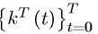 with kτ (0) = ko. Show that for every ε > 0, there exists T < ∞
 and t' < T such that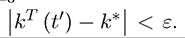 Show that kτ (T) = 0. Then assuming that ko is
sufficiently small, show that the optimal capital-labor ratio sequence looks as in Figure 6.1.
EXERCISE 6.18. Prove that as claimed in the proof of Proposition 6.3, Assumption 2 implies that s (ε) > ε for ε sufficiently small. Provide an intuition for this result.
EXERCISE 6.19. * Provide a proof of Proposition 6.1 without the differentiability assumption on the utility function u (∙) imposed in Assumption 3'.
EXERCISE 6.20. Prove that the optimal growth path starting with capital-labor ratio ko, which satisfies (6.37) is identical to the competitive equilibrium starting with capital-labor ratio and satisfying the same condition (or equivalently, equation (6.42)).