The previous chapter introduced the basic tools of dynamic optimization in discrete time.
I will now review a number of basic results in dynamic optimization in continuous time— particularly the so-called optimal control approach. Both dynamic optimization in discrete time and in continuous time are useful tools for macroeconomics and other areas of dynamic economic analysis.
One approach is not superior to another; instead, certain problems become simpler in discrete time while, certain others are naturally formulated in continuous time.Continuous-time optimization introduces a number of new mathematical issues. The main reason is that even with a finite horizon, the maximization is with respect to an infinitedimensional object (in fact an entire function, This requires a brief review
of some basic ideas from the calculus of variations and from the theory of optimal control. Most of the tools and ideas that are necessary for this book are straightforward. Nevertheless, a reader who simply wishes to apply these tools may decide skim most of this chapter, focusing on the main theorems, especially Theorems 7.14 and 7.15, and their application to the canonical continuous-time optimal growth problem in Section 7.7.
In the rest of this chapter, I first review the finite-horizon continuous-time maximization problem and provide the simplest treatment of this problem (which is more similar to calculus of variations than to optimal control). I then present the more powerful theorems from the theory of optimal control as developed by Pontryagin and co-authors.
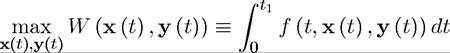
The canonical problem we are interested in can be written as
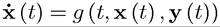
subject to
and

where for each t, x (t) and y (t) are finite-dimensional vectors and y (t) ∈
, where Kx and Ky are integers).
We refer to x as the state variable. Its behavior is governed by a vector-valued differential equation (i.e., a set of differential equations) given the behavior of the control variables y (t). The end of the planning horizon tι can be equal to infinity. The function W (x (t), y (t)) denotes the value of the objective function when controls are given by y (t) and the resulting behavior of the state variable is summarized by x (t). We also refer to f as the objective function (or the payoff function) and to g as the constraint function.This problem formulation is general enough to incorporate discounting, since both the instantaneous payoff function f and the constraint function g depend directly on time in an arbitrary fashion. We will start with the finite-horizon case and then treat the infinitehorizon maximization problem, focusing particularly on the case where there is exponential discounting.
7.1.