Variational Arguments
(7.1)
Consider the following finite-horizon continuous time problem
subject to (7.2)
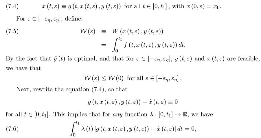
and

Here the state variable x (t) ∈ R is one-dimensional and its behavior is governed by the differential equation (7.2).
The control variable y (t) must belong to the set Ó (t) ⊂ R. Throughout, we assume that Ó (t) is nonempty and convex. We refer to a pair of functions (x (t),y (t)) that jointly satisfy (7.2) and (7.3) as an admissible pair. Throughout, as in the previous chapter, we assume the value of the objective function is finite, that is, W (x (t),y (t)) < ∞ for any admissible pair (x (t),y (t)).Let us first suppose that tι < ∞, so that we have a finite-horizon optimization problem. Notice that there is also a terminal value constraint x (tf) = xχ, but xι is included as an additional choice variable. This implies that the terminal value of the state variable x is free. Below, we will see that in the context of finite-horizon economic problems, the formulation where xι is not a choice variable may be simpler (see Example 7.1), but the development in this section is more natural when the terminal value xι is free.
In addition, to simplify the exposition, throughout we assume that f and g are continuously differentiable functions.
The difficulty in characterizing the optimal solution to this problem lies in two features:
(1) We are choosing a function y : [0,tι] → Ó rather than a vector or a finite dimensional ob ject.
(2) The constraint takes the form of a differential equation, rather than a set of inequalities or equalities.
These features make it difficult for us to know what type of optimal policy to look for. For example, y may be a highly discontinuous function. It may also hit the boundary of the feasible set—thus corresponding to a “corner solution”. Fortunately, in most economic problems there will be enough structure to make optimal solutions continuous functions. Moreover, in most macroeconomic and growth applications, the Inada conditions make sure that the optimal solutions to the relevant dynamic optimization problems lie in the interior of the feasible set. These features considerably simplify the characterization of the optimal solution. In fact, when y is a continuous function of time and lies in the interior of the feasible set, it can be characterized by using the variational arguments similar to those developed by Euler, Lagrange and others in the context of the theory of calculus of variations. Since these tools are not only simpler but also more intuitive, we start our treatment with these variational arguments.
The variational principle of the calculus of variations simplifies the above maximization problem by first assuming that a continuous solution (function) y that lies everywhere in the interior of the set Y exists, and then characterizes what features this solution must have in order to reach an optimum (for the relationship of the results here to the calculus of variations, see Exercise 7.3).
More formally let us assume that is an admissible pair such that y(∙) is
continuous over [0,tι] and , and we have
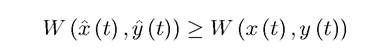
for any other admissible pair (x (t),y (t)).
The important and stringent assumption here is that (X (t),y (t)) is an optimal solution that never hits the boundary and that does not involve any discontinuities.
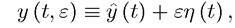
Even though this will be a feature of optimal controls in most economic applications, in purely mathematical terms this is a strong assumption. Recall, for example, that in the previous chapter, we did not make such an assumption and instead started with a result on the existence of solutions and then proceeded to characterizing the properties of this solution (such as continuity and differentiability of the value function). However, the problem of continuous time optimization is sufficiently difficult that proving existence of solutions is not a trivial matter. We will return to a further discussion of this issue below, but for now we follow the standard practice and assume that an interior continuous solution y (t) ∈IntY (t), together with the corresponding law of motion of the state variable, X (t), exists. Note also that since the behavior of the state variable x is given by the differential equation (7.2), when y (t) is continuous, X (t) will also be continuous, so that x (t) is continuously differentiable. When y (t) is piecewise continuous, x (t) will be, correspondingly, piecewise smooth.We now exploit these features to derive necessary conditions for an optimal path of this form. To do this, consider the following variation
where η (t) is an arbitrary fixed continuous function and ε ∈ R is a scalar. We refer to this as a variation, because given η (t), by varying ε, we obtain different sequences of controls. The problem, of course, is that some of these may be infeasible, i.e., y (t, ε) ∈ Ó (t) for some t. However, since y (t) ∈Inty (t), and a continuous function over a compact set [0,tι] is bounded, for any fixed η (∙) function, we can always find εη > 0 such that
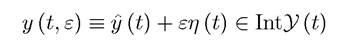
 constitutes a feasible variation.
To prepare for these arguments, let us fix an arbitrary η (∙), and define x (t, ε) as the path of the state variable corresponding to the path of control variable y (t, ε). This implies that x (t, ε) is given by:
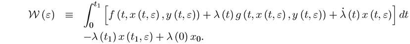
since the term in square brackets is identically equal to zero. In what follows, we suppose that the function λ (∙) is continuously differentiable. This function, when chosen suitably, will be the costate variable, with a similar interpretation to the Lagrange multipliers in standard (constrained) optimization problems. As with Lagrange multipliers, this will not be true for
any λ (∙) function, but only for a λ (∙) that is chosen appropriately to play the role of the costate variable.
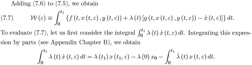
Substituting this expression back into (7.7), we obtain:
Recall that f and g are continuously differentiable, and y (t, ε) is continuously differentiable in ε by construction, which also implies that x (t, ε) is continuously differentiable in ε. Let us denote the partial derivatives of x and y by xε and yε, and the partial derivatives of f and g by ft, fx, fy, θtc..
Differentiating the previous expression with respect to ε (making use of Leibniz’s rule, Theorem B.4 in Appendix Chapter B), we obtain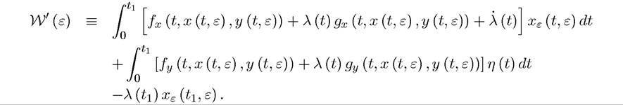
Let us next evaluate this derivative at ε = 0 to obtain:
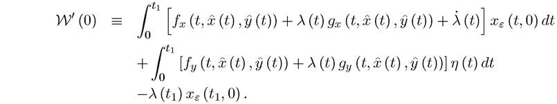
where, as above, x (t) = x (t, ε = 0) denotes the path of the state variable corresponding to the optimal plan, y (t). As with standard finite-dimensional optimization, if there exists some function η (t) for which W0 (0) = 0, this means that W (x (t),y (t)) can be increased and thus the pair (x (t),y(t)) could not be an optimal solution. Consequently, optimality requires that

Recall that the expression for ) applies for any continuously differentiable λ (t) function. Clearly, not all such functions λ (∙) will play the role of a costate variable. Instead, as it is 263
the case with Lagrange multipliers, the function λ (∙) has to be chosen appropriately, and in this case, it must satisfy
while the third term will be equal to zero for all values of xε (tχ, 0), if and only if λ (tχ) = 0. The last two steps are further elaborated in Exercise 7.1. We have therefore obtained the result that the necessary conditions for an interior continuous solution to the problem of maximizing (7.1) subject to (7.2) and (7.3) are such that there should exist a continuously differentiable function λ (∙) that satisfies (7.9), (7.10) and λ (tχ) = 0.
The condition that λ (tχ) = 0 is the transversality condition of continuous time optimization problems, which is naturally related to the transversality condition we encountered in the previous chapter.
Intuitively, this condition captures the fact that after the planning horizon, there is no value to having more x.This derivation, which builds on the standard arguments of calculus of variations, has therefore established the following theorem.[14]
Theorem 7.1. (Necessary Conditions) Consider the problem of maximizing (7.1) subject to (7.2) and (7.3), with f and g continuously differentiable. Suppose that this problem has an interior continuous solution y (t) ∈Inty (t) with corresponding path of state variable x(t). Then there exists a continuously differentiable costate function λ (∙) defined over t ∈ [0,tχ] such that (7.2), (7.9) and (7.10) hold, and moreover λ (tχ) = 0.
As noted above, (7.9) looks similar to the first-order conditions of the constrained maximization problem, with λ (t) playing the role of the Lagrange multiplier. We will return to this interpretation of the costate variable λ (t) below.
Let ns next consider a slightly different version of Theorem 7.1, where the terminal value of the state variable, xχ, is fixed, so that the maximization problem is 
subject to (7.2) and (7.3). The only difference is that there is no longer a choice over the terminal value of the state variable, xi. In this case, we have:
Theorem 7.2. (Necessary Conditions II) Consider the problem of maximizing (7.11) subject to (7.2) and (7.3), with f and g continuously differentiable. Suppose that this problem has an interior continuous solution y (t) ∈Inty (t) with corresponding path of state variable x(t). Then there exists a continuously differentiable costate function λ (∙) defined over t ∈ [0,tι] such that (7.2), (7.9) and (7.10) hold.
Proof. The proof is similar to the arguments leading to Theorem 7.1, with the main change that now x (tι,ε) must equal xi for feasibility, so xε (ti, 0) = 0 and λ (tι) is unrestricted. Exercise 7.5 asks you to complete the details. ?
The new feature in this theorem is that the transversality condition λ (ti) = 0 is no longer present, but we need to know what the terminal value of the state variable x should be.* [15] [16] We first start with an application of the necessary conditions in Theorem 7.2 to a simple economic problem. More interesting economic examples are provided later in the chapter and in the exercises.
EXAMPLE 7.1. Consider a relatively common application of the techniques developed so far, which is the problem of utility-maximizing choice of consumption plan by an individual that lives between dates 0 and 1 (perhaps the most common application of these techniques is a physical one, that of finding the shortest curve between two points in the plane, see Exercise 7.4). The individual has an instantaneous utility function u (c) and discounts the future exponentially at the rate p > 0. We assume that is a strictly increasing,
continuously differentiable and strictly concave function. The individual starts with a level of assets equal to a (0) > 0, earns an interest rate r on his asset holdings and also has a constant flow of labor earnings equal to w. Let us also suppose that the individual can never have negative asset position, so that a (t) ≥ 0 for all t. Therefore, the problem of the individual can be written as
subject to
and a (t) ≥ 0, with an initial value of a (0) > 0. In this problem, consumption is the control variable, while the asset holdings of the individual are the state variable.
To be able to apply Theorem 7.2, we need a terminal condition for a (t), i.e., some value ai such that a (1) = αt. The economics of the problem makes it clear that the individual would not like to have any positive level of assets at the end of his planning horizon (since he could consume all of these at date t = 1 or slightly before, and u (∙) is strictly increasing). Therefore, we must have a (1) = 0.
With this observation, Theorem 7.2 provides the following the necessary conditions for an interior continuous solution: there exists a continuously differentiable costate variable λ (t) such that the optimal path of consumption and asset holdings, (c(t), a (t)), satisfy a consumption Euler equation similar to equation (6.29) in Example 6.5 in the previous chapter:

In particular, this equation can be rewritten as u' (c(t)) = βrλ (t), with β = exp (—ρt), and would be almost identical to equation (6.29), except for the presence of λ (t) instead of the derivative of the value function. But as we will see below, λ (t) is exactly the derivative of the value function, so that the consumption Euler equations in discrete and continuous time are identical. This is of course not surprising, since they capture the same economic phenomenon, in slightly different mathematical formulations.
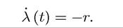
The next necessary condition determines the behavior of λ (t) as
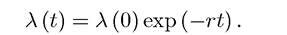
Now using this condition and differentiating u' (c(t)) = βrλ (t), we can obtain a differential equation in consumption. This differential equation, derived in the next chapter in a somewhat more general context, will be the key consumption Euler equation in continuous time. Leaving the derivation of this equation to the next chapter, we can make progress here by simply integrating this condition to obtain
Combining this with the first-order condition for consumption yields a straightforward expression for the optimal consumption level at time t:

where is the inverse function of the marginal utility u'. It exists and is strictly decreasing in view of the fact that u is strictly concave. This equation therefore implies that when ρ = r, so that the discount factor and the rate of return on assets are equal, the individual will have a constant consumption profile. When p > r, the argument of u'-1 is increasing over time, so consumption must be declining. This reflects the fact that the individual discounts the future more heavily than the rate of return, thus wishes to have a 266
front-loaded consumption profile. In contrast, when p since λ (1) = 0, this is only possible if λ (t) = 0 for all t ∈ [0,1]. But then the Euler equation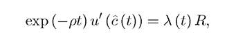
which still applies from the necessary conditions, cannot be satisfied, since u' > 0 by assumption. This implies that when the terminal value of the assets, a (1), is a choice variable, there exists no solution (at least no solution with an interior continuous control). How is this possible?
The answer is that Theorem 7.1 cannot be applied to this problem, because there is an additional constraint that a (t) ≥ 0. We would need to consider a version of Theorem 7.1 with inequality constraints. The necessary conditions with inequality constraints are messier and more difficult to work with. Using a little bit of economic reasoning to observe that the terminal value of the assets must be equal to zero and then applying Theorem 7.2 simplifies the analysis considerably.
7.2.