Financial Development

An important aspect of the structural transformation brought about by economic devel­opment is a change in financial relations and deepening of financial markets. Section 17.6 in Chapter 17 already presented a model where economic growth goes hand-in-hand with finan­cial deepening.

and relaxation of credit market constraints might lead to better income and risk sharing. On the other hand, as the possibility of such risk-sharing arrangements reduce consumption risk, individuals might also take riskier actions, potentially affecting the distribution of income. A complete analysis of the issues surrounding financial development and its interactions with economic growth are beyond the scope of this chapter.

Here I will instead present a simple model of financial development, focusing on the diversification of idiosyncratic risks and complementing the analysis in Section 17.6. The model is inspired by the work of Townsend (1979) and Greenwood and Jovanovic (1990) and adopts some of the modeling features of the model of Acemoglu and Zilibotti (1997) in Section

17.6. It will illustrate how financial development takes place endogenously and interacts with economic growth, and will also provide some simple insights about the implications of financial development for income distribution. Given the similarity of the model to that in Section

17.6, my treatment here will be relatively quick and informal.

I consider an overlapping generations economy in which each individual lives for two periods and has preference given by

where c (t) denotes the consumption of the unique final good of the economy and E_t denotes the expectation operator given time t information. As we already seen Chapter 9 and also in Section 17.6, these preferences are very convenient since they ensure a constant savings rate.

There is no population growth and the total population of each generation is normalized to 1. Let us assume that each individual is born with some labor endowment l. The distribution of endowments across agents is given by the distribution function G (l) over some support [l, Z] This distribution of labor endowments is constant over time with mean L = 1 and labor is supplied inelastically by all individuals in the first period of their lives.

The aggregate production function of the economy is given by

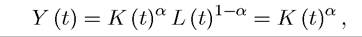
where α ∈ (0,1) and the second equality uses the fact that total labor supply will be equal to 1 at each date. As in Section 17.6, the only risk is in transforming savings into capital, thus the lifecycle of an individual looks identical to that shown in Figure 17.3 in that section.

852

Moreover, we assume that agents can either save all of their labor earnings from the first period of their lives using a safe technology with rate of return q (in terms of capital at the next date) or invest all of their labor income in the risky technology with return Q + ε, where ε is a mean zero independently and identically distributed stochastic shock and

This implies that the risky technology is more productive. The assumption that individuals have to choose one of these two technologies rather than dividing their savings between the two is made for simplicity only (see Exercise 21.1).

Although the model looks very similar to that in Section 17.6, there is a crucial difference. Because ε is identically and independently distributed across individuals, if individuals could pool their resources, they would get rid of the idiosyncratic risk and enjoy the higher return Q. In particular, if a large number (a continuum) all individuals pooled their resources, they would guarantee an average return of Q. Let us assume that this is not possible because of a standard informational problem—the actual return of an individual’s saving decision is not observed by other individuals unless some financial monitoring is undertaken. Let us assume that this type of financial monitoring has a cost ξ > 0 for each individual.

If the individual does not join the financial markets, then no other agent in the economy can observe the realization of the returns on his savings. In this case, no financial contract for sharing of idiosyncratic risks is possible, since such a contract would involve agents that have a high (realized) value of ε making transfers to those who are unlucky and have low realized values of ε. However, without monitoring, each agent will claim to have a low value of ε, thus receive rather than make ex post payments. The anticipation of this type of opportunistic behavior prevents any risk sharing in the absence of monitoring.

Let us also assume that ε has a distribution that places positive probability on ε = -Q. This implies that if an individual undertakes the risky investments, there is a positive probability that all his savings will be lost. This immediately implies that without some type of risk sharing, individuals would always choose the safe project. This observation 853

significantly simplifies the analysis of the model. Now suppose that the economy starts with some initial capital stock of K (0). This implies that an individual with labor endowment Ö will have labor earnings of

where

id="Picutre 2724" class="lazyload" data-src="/files/uch_group77/uch_pgroup317/uch_uch7364/image/image2722.jpg">

is the competitive wage rate at time t. After labor incomes are realized, individuals first make their savings decisions and then choose which assets to invest in.

of their income regardless of their income level or the rate of return (in particular, independent of whether they are investing in the risky or the safe asset). In view of this, the value to not participating in the financial markets for individual i at time t is

which takes into account that the rate of return on capital in the second period of the life of the individual will be R (t + 1) and the individual will receive a gross return q on his savings of βWi (t) / (1 + β). In contrast, when the individual decides to take part in financial markets (presuming that there are sufficiently many other individuals also taking part in financial markets to provide risk diversification, which here means a positive measure of individuals doing so), his value will be

which takes into account that the individual will have to spend the amount ξ out of his labor income on the cost of joining the financial market, leaving him a net income of Wi (t) — ξ. He will then save a fraction β/ (1 + β) of this, but in return, he will receive the higher gross return Q. The reason why the individual will necessarily receive Q, rather than a risky return, is because, conditional on joining the financial market, each individual is able to fully diversify his idiosyncratic risks and therefore receive the average return Q. The comparison

of these two expressions immediately gives the threshold level

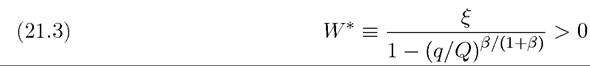
such that individuals with first-period earnings greater than W^* will join the financial market and those with less than W^* will not.

independent of the rate of return on capital in the second period of the lives of the individuals, R. This is an implication of log preferences in (21.1).

Now that we have determined the behavior of individuals concerning whether they will join the financial market, we can determine the evolution of the economy by studying the evolution of individual earnings. Individual earnings are determined by two factors: individ­ual labor endowments and the capital stock at time t, which determines the wage per unit of labor, w (t), as given in (21.2). In particular, suppose that at time t the wage is given by w (t). Then the fraction of individuals who will join the financial market at time t, g^F (t), is given by the fraction of individuals who have li ≥ W*/w (t). Alternatively, using the fact that labor endowments have a distribution given by G (∙), the fraction of individuals investing in financial markets is obtained as

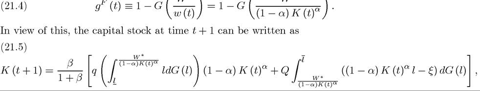
which takes into account that all individuals with labor endowment less than

W*/q (1 — α) K (t)^α will choose the safe project and receive the gross return q on their sav­ings, while those above this threshold will spend ξ on the fixed cost of monitoring and then receive the higher return Q. It can be verified that K (t + 1) is increasing in K (t) and there will be growth in the capital stock (and thus output) of the economy provided that K (t) is small enough (in particular, less than the “steady-state” level of capital when this is unique; see Exercise 21.2).

Now inspection of the accumulation equation (21.5) together with the threshold rule for joining the financial market leads to a number of interesting conclusions.

(1) As K (t) increases, that is, as the economy develops, equation (21.4) implies that more individuals will join the financial market. Consequently, a greater level of capital will lead to more risk taking, but these risks will also be shared better. More importantly, economic development also induces a better composition of investment as a greater fraction of the individuals start using their savings more efficiently. Thus with a mechanism similar to the model in Section 17.6, economic development leads to endogenously higher productivity by improving the allocation of funds in the economy. Consequently, this model, like the one in Section 17.6, implies that economic development and financial development go hand-in-hand.

(2) However, there is also a distinct sense in which the economy here allows for a po­tential causal effect of financial development on economic growth. Imagine that

societies differ according to their ξs, which can be interpreted as a measure of the institutionally- or technologically-determined costs of monitoring or some cost of fi­nancial transactions that depend on the degree of investor protection. Societies with lower ξs will have a greater participation in financial markets and this will endoge­nously increase their productivity. Thus while the equilibrium behavior of financial and economic development are jointly determined, differences in financial develop­ment driven by exogenous institutional factors related to ξ will have a potential causal effect on economic growth.

(3) As noted above, at any given point in time it will be the richer agents—those with greater labor endowment—that will join the financial market. Therefore, initially, the financial market will help those who are already well-off to increase the rate of return on their savings. This can be thought of as the unequalizing effect of the financial market.

(4) The fact that participation in financial market increases with K (t) also implies that as the economy grows, at least at the early stages of economic development, the unequalizing effect of financial intermediation will become stronger. Therefore, presuming that the economy starts with relatively few rich individuals, the first expansion of the financial market will increase the level of overall inequality in the economy as a greater fraction of the agents in the economy now enjoy the greater returns.

(5) As K (t) increases even further, eventually the equalizing effect of the financial mar­ket will start operating. At this point, the fraction of the population joining the financial market and enjoying the greater returns is steadily increasing. If the steady­state level of capital stock K* is such that l ≥ W*/ (1 — α)(K*)^α, then eventually all individuals will join the financial market and they will all receive the same rate of return on their savings.

The last two observations are interesting in part because the relationship between growth and inequality is a topic of great interest to development economics (one to which we will return later in this chapter). One of the most important ideas in this context is that of the Kuznets curve, based on Simon Kuznets’s observations, which claims that growth first increases income inequality in the society and then leads to a decline in inequality. Whether or not the Kuznets curve is a good description of the relationship between growth and inequality is a topic of current debate. While many European societies seem to have gone through a phase of increasing and then decreasing inequality during the growth process over the 19th century, the evidence for the 20th century is more mixed. Nevertheless, the last two observations show that a model with endogenous financial development based on risk sharing among individuals can generate a pattern consistent with the Kuznets curve. Whether there 856

is indeed a Kuznets curve in general and if so, whether the mechanism highlighted here plays an important role in generating this pattern are areas for future theoretical and empirical work.

21.2.