Fertility, Mortality and the Demographic Transition
Chapter 1 highlighted the big questions related to growth of income per capita over time and its dispersion across countries today. Our focus so far has been on these per capita income differences.
Equally striking differences exist in the level of population across countries and over time. Figure 21.1 uses data from Maddison (2002) and shows the levels and the evolution of population in different parts of the world over the past 2000 years. The figure is in log scale, so a linear curve indicates a constant rate of population growth. The figure shows that starting about 250 years ago there is a significant increase in the population growth rate in many areas of the world. This accelerated population growth continues in much of the world, but importantly, the rate of population growth slows down in Western Europe sometime in the 19th century (though not so in the Western Offshoots because of immigration). There is no similar slow down of population growth in less-developed parts of the world. On the contrary, in many less developed nations, the rate of population growth seems to have increased over the past 50 or so years. We have already discussed one of the reasons for this in Chapter 4— the spread of antibiotics, basic sanitation and other health-care measures around the world that reduced the very high mortality rates in many countries. However, equally notable is the demographic transition in Western Europe, which is the term coined for the decline in fertility sometime during the 19th century (more precisely at different points during this century for different countries). Understanding why population has grown slowly and then accelerated to reach a breakneck speed of growth over the past 150 years and why population growth rates differ across countries are major questions for economic development and economic growth. These questions are not only interesting because population levels are among the variables we would like to understand and explain, but also because one might sometimes wish to focus on differences in total income across societies rather than on income per capita differences. In this case, differences in population become a variable to focus on directly.In this section, I discuss the most basic approaches to population dynamics and fertility. I first discuss a simple version of the famous Malthusian model and then use a variant of this model to investigate potential causes of the demographic transition. This is a vast and important area of research and one section can hardly do justice to the important empirical and theoretical issues. Thomas Malthus was one of the most brilliant and influential economists of the 19th century and is responsible for one of the first general equilibrium growth models. The next subsection will present a version of this model. The Malthusian model is responsible for earning the discipline of economics the name “the dismal science” because 857
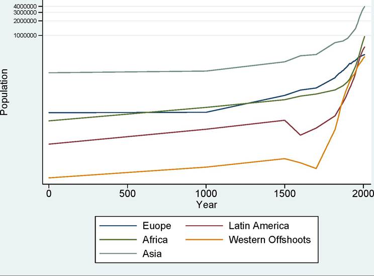
Figure 21.1. Total population in different parts of the world over the past 2000 years.
of its dire prediction that population will adjust up or down (by births or deaths) until all individuals are at the subsistence level of consumption. Nevertheless, this dire prediction is not the most important part of the Malthusian model. Instead, at the heart of this model is the negative relationship between population, which is itself endogenously determined, and income per capita. In this sense, it is closely related to the Solow model or the neoclassical growth model, augmented with a behavioral rule that determines the rate of population growth. It is this less extreme version of the Malthusian model that will be presented in the next subsection. I will then enrich this model by the important and influential idea due to Gary Becker that there is a tradeoff between the quantity and quality of children and that this tradeoff changes over the process of development. I will show how a simple model can capture the process via which parents start valuing the quality (human capital) of their offsprings more as the economy becomes richer and demands more human capital.
This process will eventually lead to the demographic transition, with fewer but more skilled children. Since my ob jective here is to introduce the main ideas rather than give a full account of this active research area, my treatment will be informal.21.2.1. A Simple Malthusian Model. Consider the following non-overlapping generations model. We start with a population of L (0) > 0 at time t = 0. Each individual living at time t supplies one unit of labor inelastically and has preferences given by

where c (t) denotes the consumption of the unique final good of the economy by the individual himself, n (t + 1) denotes the number of offsprings the individual has and ó (t + 1) is the income of each offspring, and β > 0 and ηo > 0. The last term in square brackets is the childrearing costs and are assumed to be convex to reflect the fact that the costs of having more and more children will be higher (for example, because of time constraints of parents, though one can also make arguments for why the costs of child-rearing might exhibit increasing returns to scale over a certain range). Clearly, these preferences introduce a number of simplifying assumptions. First, each individual is allowed to have as many offsprings as it likes, which is unrealistic because it does not restrict the number of offsprings to an integer. The technology also does not incorporate possible specialization in child-rearing and market work within the family. Second, these preferences introduce the “warm glow” type altruism we encountered in Chapter 9, so that parents receive utility not from the utility of their offspring, but from some characteristic of their offsprings. Here it is a transform of the total income of all the offsprings that features in the utility function of the parent. Third, the costs of child-rearing are in terms of “utils” rather than forgone income and current consumption multiplies both the benefits and the costs of having additional children.
This feature, which is motivated by balanced growth type reasoning, implies that the demand for children will be independent of current income (otherwise, growth will automatically lead to greater demand for children). All three of these assumptions are for simplicity and do not have important effects on the main insights of the model, though they naturally change many of the key expressions and some of the auxiliary implications. I have also written the number of offsprings that an individual has a time t as n (t + 1), since this will determine population at time t + 1.Each individual has one unit of labor and there are no savings. The production function for the unique good takes the form

where Z is the total amount of land available for production and L (t) is total labor supply. There is no capital and land is introduced in order to create diminishing returns to labor, which is an important element of the Malthusian model. I normalize the total amount of land to Z = 1 without loss of any generality. A key question in models of this sort is what happens to the returns to land. The most satisfactory way of dealing with this problem would be to allocate the property rights to land among the individuals and let them bequeath this 859
to their offsprings. This, however, introduces another layer of complication, and since my purpose here is to illustrate the basic ideas, I will follow the unsatisfactory assumption often made in the literature, that land is owned by another set of agents, whose behavior will not be analyzed here. The main important assumption made here is that those receiving land rents do not supply labor and/or their offsprings do not make an important contribution to overall population growth.
By definition, population at time t + 1 is given as
(21.8) L (t + 1) = n (t + 1) L (t),
which takes into account new births as well as the death of the parent.
L(t+1)
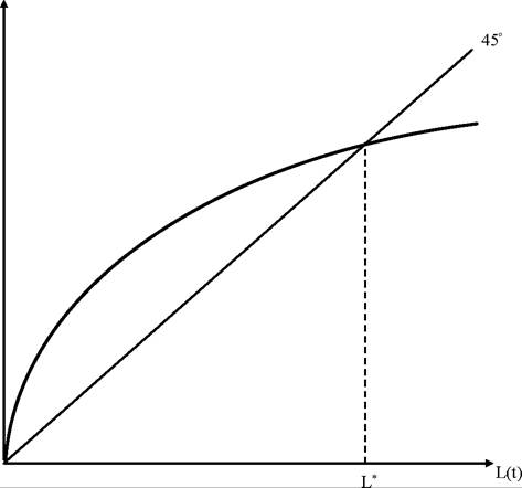
FIGURE 21.2. Population dynamics in this simple Malthusian model.
Labor markets are competitive, so the wage at time t + 1 is given as

Since there is no other source of income, this is also equal to the income of each individual living at time t + 1, y (t + 1). Thus an individual with income w (t) at time t will solve the problem of maximizing (21.6) subject to the constraint that c (t) ≤ w (t), together with 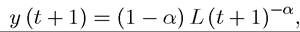 which implies that the individual takes the population level in the next period as given (since he is infinitesimal). Let us focus on a symmetric equilibrium, which will naturally require the choice of n (t + 1) to be consistent with L (t + 1) according 860
to equation (21.8). This maximization problem immediately gives c (t) = w (t) and
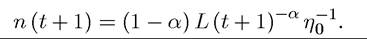
Now substituting for (21.8) and rearranging, we obtain

This equation implies that L (t + 1) is an increasing concave function of L (t). In fact, the law of motion for population implied by (21.10) resembles the dynamics of capital-labor ratio in the Solow growth model (or the overlapping generations model) and is plotted in Figure
21.2. The figure makes it clear that starting with any L (0) > 0, there exists a unique globally stable state state L* given by

If the economy starts with L (0) < L*, then population will slowly (and monotonically) adjust towards this steady-state level. Moreover, (21.9) shows that as population increases wages will fall.
If in contrast, L (0) > L*, then the society will experience a decline in population and rising real wages. It is straightforward to introduce shocks to population and show that in this case the economy will fluctuate around the state-state population level L* (with an invariant distribution depending on the distribution of the shocks) and experience cycles reminiscent to the Malthusian cycles, with periods of increasing population and decreasing wages followed by periods of decreasing population and increasing wages (see Exercise 21.3). The main difference of this model from the simplest (or the crudest) version of the Malthusian model is that there is no biologically determined subsistence level of consumption. The level of consumption will tend to a constant given by
though this is not determined biologically, but by preferences and technology.
21.2.2. The Demographic Transition. I now extend the basic Malthusian model of the previous subsection in two respects to study the demographic transition. First, I introduce a quality-quantity tradeoff along the lines of the ideas suggested by Gary Becker. Each parent can choose his offsprings to be unskilled or skilled. To make them skilled, the parent has to exert the additional effort for child-rearing denoted by e (t) ∈ {0,1}. If he chooses not to do this, his offsprings will be unskilled.
The total population of unskilled individuals at time t is denoted by U (t) and the total population of the skilled are denoted by S (t), clearly with
861
The second modification is that there are now two production technologies that can be used for producing the final good. The Malthusian (traditional) technology is still given by (21.7) and any worker can be employed with the Malthusian technology. The modern technology is given by

This equation implies that productivity in the modern technology is potentially time varying and also states that only skilled workers can be employed with this technology. It also imposes that all skilled workers will be employed with this technology. Naturally, this need not be true in general (there may be an excess supply of skilled workers). However, this will never be the case in equilibrium, since parents would not choose to exert the additional effort to endow their offsprings with skills if they would then work in the traditional sector. In the interest of keeping the exposition brief and simple (and with a slight abuse of notation), equation (21.12) already incorporates the fact that all skilled workers will be employed in the modern sector.
To incorporate the quality-quantity tradeoff, individual preferences are now modified from 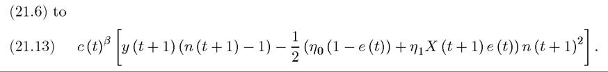 This formulation of the preferences states that if the individual decides invests in his offsprings’ skills, instead of the fixed cost η0 he has to pay a cost that is proportional to the amount of knowledge X (t + 1) that the offspring has to absorb to use the modern technology. I assume that X (0) η1 > η0, so that even at the initial level of the modern technology rearing a skilled child is more costly than an unskilled child.
Finally, I make the same external learning-by-doing assumption as in Romer (1986) or the model of industrialization in Section 20.3, and assume that

which implies that the improvement in the technology of the modern sector is a function of the number of skilled workers employed in this sector. This type of reduced form assumption is clearly unsatisfactory, but as noted above, one could get similar results with an endogenous technology model with the market size effect. Another important feature of this production function is that it does not use land. This assumption is consistent with the fact that most modern production processes make little use of land, instead relying on technology, physical capital and human capital. Equation (21.12) captures this in a simple form, though it does so without introducing physical capital.
The output of the traditional and the modern sector are perfect substitutes—they both produce the same final good. In view of the observation that all unskilled workers will work 862
in the traditional sector and all skilled workers will work in the modern sector, we have wages of skilled and unskilled workers at time t as

and

where (21.15) is identical to (21.9) in the previous subsection, except that it features only the unskilled workers instead of the entire labor force.
Let us next turn to the fertility and quality-quantity decisions of individuals. As before, each individual will consume all his income and his income level has no effect on his fertility and quality-quantity decisions. Thus we do not need to distinguish between high-skill and low- skill parents. Using this observation, let us simply look at the optimal number of offsprings that an individual will have when he chooses e (t) = 0. This is given by
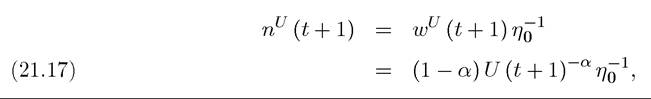
where the second line uses (21.15). Instead, if the parent decides to exert effort e (t) = 1 and invest in the skills of his offsprings, then he will choose the number of offsprings equal to
The comparison of equations (21.17) and (21.18) suggests that unless unskilled wages are very low, an individual who decides to provide additional skills to his offsprings will have fewer offsprings. This is because bringing up skilled children is more expensive. Thus the comparison of these two equations captures the quality-quantity tradeoff.
Now substituting these equations back into the utility function (21.13), we obtain the utility from the two strategies (normalized by consumption, which does not affect his decision)
Inspection of these two expressions shows that we can never have an equilibrium in which all offsprings are skilled, since otherwise Vu would become unboundly large. Therefore, in equilibrium we must have
863
This equilibrium condition implies that there are two possible configurations. First, X (0) can be so low that (21.19) will hold as a strict inequality. In this case, all offsprings will be unskilled. The condition for this inequality to be strict is
which uses the fact that when there are no skilled workers there is no production in the modern sector and thus X (1) = X (0). If this inequality satisfied, there would be no skilled children at date t = 0. However, as long as L (1) is less than L* as given in (21.11), population will grow. It is therefore possible that at some point (21.19) holds with equality. The condition for this never to happen is that

In this case, the law of motion of population is identical to that in the previous subsection and there is never any investment in skills. We can think of this is a pure Malthusian economy.
If, on the other hand, this condition is not satisfied, then at least at some point individuals will start investing in the skills of their offsprings and the modern sector will have skilled workers to employ. From then on (21.19) must hold as equality. In that case, let the fraction of parents having unskilled children at time t be denoted by u (t + 1). Then by definition 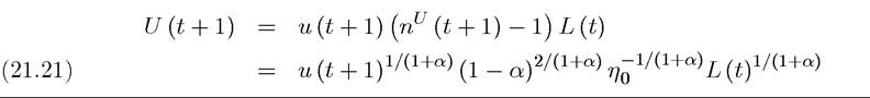 and
and
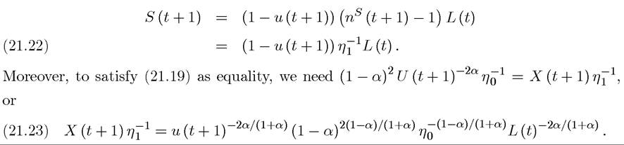
Equilibrium dynamics are then determined by equations (21.21)-(21.23) together with (21.16). While the details of the behavior of this dynamical system are somewhat involved, the general picture is clear. If an economy starts with both a low level of X (0) and a low level of L (0), but does not satisfy condition (21.20), then the economy will start in the Malthusian regime, only making use of the traditional technology and not investing in skills. As population increases wages fall, and at that point parents start finding it beneficial to invest in the skills of their children and firms start using the modern technology. Those parents that invest in the skills of their children have fewer children than parents rearing unskilled offsprings. The rate of population growth and fertility are high at first, but as the modern technology improves and the demand for skills increases, a larger fraction of the parents start investing 864
in the skills of their children and the rate of population growth declines. Ultimately, the rate of population growth approaches η-1. Thus this model gives a very stylized representation of the demographic transition.
In the literature, there are richer models of the demographic transition. For example, there are many ways of introducing quality-quantity tradeoffs in the utility function of the parents, and what spurs a change in the quality-quantity tradeoff may be an increase in capital intensity of production, changes in the wages of workers, or even changes in the wages of women differentially affecting the desirability of market and home activities. Nevertheless, the general qualitative features are similar in that the quality-quantity tradeoff is often viewed as the ma jor reason for the demographic transition. Despite this emphasis on the qualityquantity tradeoff, there is relatively little direct evidence that this tradeoff is important in general or in leading to the demographic transition. Other social scientists have suggested social norms, the large declines in mortality, or the reduced need for child labor as potential factors contributing to the demographic transition. As of yet, there is no general consensus on the causes of the demographic transition or on the role of the quality-quantity tradeoff in determining population dynamics. The study of population growth and demographic transition is an exciting and important area, and theoretical and empirical analyses of the factors affecting fertility decisions and how they interact with the allocation of workers across different tasks (sectors) remain important and interesting questions to be explored.
21.3.