A First Look at Optimal Growth in Continuous Time
In this section, we briefly show that the main theorems developed so far apply to the problem of optimal growth, which was introduced in Chapter 5 and then analyzed in discrete time in the previous chapter.
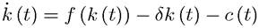
We will not provide a full treatment of this model here, since this is the topic of the next chapter.Consider the neoclassical economy without any population growth and without any technological progress. In this case, the optimal growth problem in continuous time can be written as:
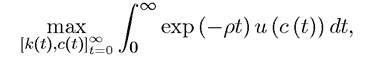
subject to
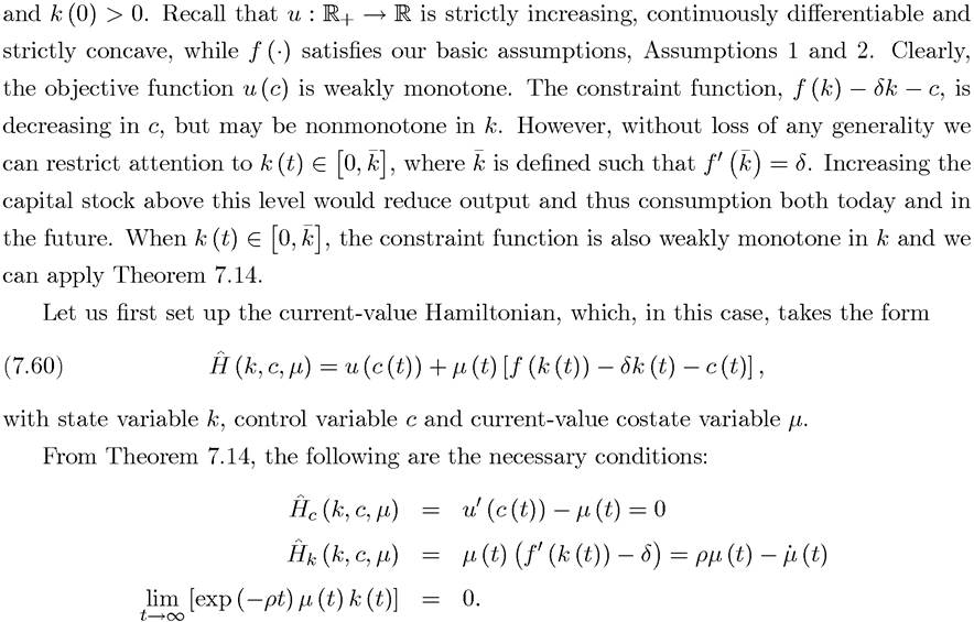
Moreover, the first necessary condition immediately implies that μ (t) > 0 (since u > 0 everywhere). Consequently, the current-value Hamiltonian given in (7.60) consists of the sum of two strictly concave functions and is itself strictly concave and thus satisfies the conditions of Theorem 7.15. Therefore, a solution that satisfies these necessary conditions in fact gives a global maximum. Characterizing the solution of these necessary conditions also establishes the existence of a solution in this case.
Since an analysis of optimal growth in the neoclassical model is more relevant in the context of the next chapter, we do not provide further details here.
7.8.