Flows into and out of Employment, Equilibrium Unemployment, and the Beveridge Curve
The model assumes that some proportion of existing jobs are terminated at every instant. The destruction of jobs and the flow from employment to unemployment are due to either cyclical or structural real disturbances that make the jobs unprofitable.
It is assumed that at any instant, the probability of destruction of any job is equal to λ, where λ is an exogenous parameter.3In contrast, job creation occurs when a firm and an employee agree to sign a contract with a wage that is the result of a bilateral negotiation. This leads to a flow out of unemployment.
Therefore, at any given moment, there are two flows in the labor market. One flow is from existing jobs to unemployment (because of job terminations), and the other is from unemployment to newly created jobs. The change of the unemployment rate is thus described by

The change in the unemployment rate at each point in time depends on the difference between the proportion of jobs destroyed and the proportion of new jobs created, the proportions being defined relative to the labor force.
In the steady state, the unemployment rate will be constant. Consequently, the equilibrium unemployment rate is determined by the condition
alt=eq18-7.png>
which implies that

which is the first key equation of this model. The equilibrium unemployment rate depends positively on λ, the exogenous rate of job destruction, and negatively on labor market tightness θ. Labor market tightness is an endogenous variable in this model and is determined in the labor market.
The negative relationship that (18.8) implies between the unemployment rate and labor market tightness θ (or equivalently, between the unemployment rate and the vacancy rate) is usually called the Beveridge curve and is depicted in figure 18.1.4
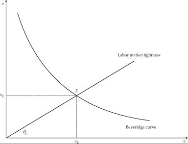
Figure 18.1 The Beveridge curve and equilibrium unemployment.
The Beveridge curve only defines a negative relation between vacancies and unemployment. For unemployment to be determined, one needs to determine labor market tightness, which is one of the endogenous variables in this model. Once labor market tightness is determined, then equilibrium unemployment is determined by the Beveridge curve. For example, assume that labor market tightness is equal to θE. Then the equilibrium unemployment rate would be determined at uE, as shown in figure 18.1.
We next turn to analyzing how the behavior of firms and unemployed job seekers results in the endogenous determination of labor market tightness.
18.3