Goods Market Equilibrium

Explain the factors

_r'., In Chapter 3 we showed that the quantity of goods and services supplied in an

affecting goods

^gg economy depends on the level of productivity—as determined, for example, by

^{market eq}U^ilibriUm.

The goods market is in equilibrium when the aggregate quantity of goods supplied equals the aggregate quantity of goods demanded. (For brevity, we refer only to "goods" rather than to "goods and services," but services always are included.) Algebraically, this condition is

(4.7)

The left side of Eq. (4.7) is the quantity of goods, Y, supplied by firms, which is determined by the factors discussed in Chapter 3.

The goods market equilibrium condition is different in an important way from the income-expenditure identity for a closed economy, Y = C + I + G (this identity is Eq. 2.3, with NX = 0). The income-expenditure identity is a relationship between actual income (output) and actual spending, which, by defi­nition, is always satisfied. In contrast, the goods market equilibrium condition does not always have to be satisfied. For example, firms may produce output faster than consumers want to buy it so that undesired inventories pile up in firms' warehouses. In this situation, the income-expenditure identity is still sat­isfied (because the undesired additions to firms' inventories are counted as part of total spending—see Chapter 2), but the goods market wouldn't be in equilib­rium because production exceeds desired spending (which does not include the

in mortgage payments, for example). As for other types of capital, constructing an apartment building is profitable only if its expected future marginal product is at least as great as its user cost.

undesired increases in inventories). Although in principle the goods market equi­librium condition need not always hold, strong forces act to bring the goods mar­ket into equilibrium fairly quickly.

A different, but equivalent, way to write the goods market equilibrium condi­tion emphasizes the relationship between desired saving and desired investment. To obtain this alternative form of the goods market equilibrium condition, we first subtract C^d + G from both sides of Eq. (4.7):

Y - C^d - G = I^d.

The left side of this equation, Y — C^d — G, is desired national saving, S^d (see Eq.

S^d = I^d. (4.8)

This alternative way of writing the goods market equilibrium condition says that the goods market is in equilibrium when desired national saving equals desired investment.

Because saving and investment are central to many issues we present in this book and because the desired-saving-equals-desired-investment form of the goods market equilibrium condition often is easier to work with, we use Eq. (4.8) in most of our analyses. However, we emphasize once again that Eq. (4.8) is equivalent to the condition that the supply of goods equals the demand for goods, Eq. (4.7).

The Saving-Investment Diagram

For the goods market to be in equilibrium, then, the aggregate supply of goods must equal the aggregate demand for goods, or equivalently, desired national saving must equal desired investment. We demonstrate in this section that adjust­ments of the real interest rate allow the goods market to attain equilibrium.^[67]

The determination of goods market equilibrium can be shown graphically with a saving-investment diagram (Figure 4.8), which shows the amount of funds supplied by savers and the amount of funds demanded by firms for investment. The real interest rate is measured along the vertical axis, and national saving and investment are measured along the horizontal axis. The saving curve, S, shows the relationship between desired national saving and the real interest rate. The upward slope of the saving curve reflects the empirical finding (Section 4.1) that a higher real interest rate raises desired national saving. The investment curve, I, shows the relationship between desired investment and the real interest rate. The investment curve slopes downward because a higher real interest rate increases the user cost of capital and thus reduces desired investment.

Goods market equilibrium is represented by point E, at which desired national saving equals desired investment, as required by Eq.

How does the goods market come to equilibrium at E, where the real interest rate is 6%? Suppose instead that the real interest rate is 3%. As Fig. 4.8 shows, when the real interest rate is 3%, the amount of investment that firms want to

FIGURE 4.8

Goods market equilibrium

Goods market equilib­rium occurs when desired national saving equals desired invest­ment. In the figure, equilibrium occurs when the real interest rate is 6% and both desired national saving and desired investment equal 1000. If the real interest rate were, say, 3%, desired investment (1500) would not equal desired national saving (850), and the goods market would not be in equilibrium. Competition among borrowers for funds would then cause the real interest rate to rise until it reaches 6%.

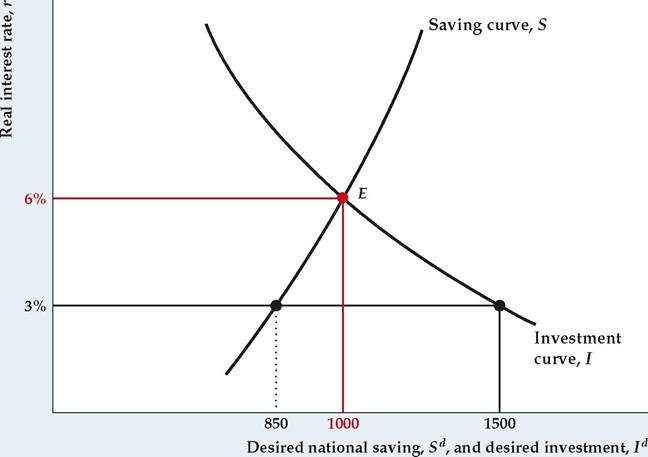
undertake (1500) exceeds desired national saving (850). With investors wanting to borrow more than savers want to lend, the "price" of funds—the real interest rate that lenders receive—will be bid up. The return to savers will rise until it reaches 6%, and desired national saving and desired investment are equal. Similarly, if the real interest rate exceeds 6%, the amount that savers want to lend will exceed what investors want to borrow, and the real return paid to savers will be bid down. Thus adjustments of the real interest rate, in response to an excess supply or excess demand for funds, bring the goods market into equilibrium.

Although Fig. 4.8 shows goods market equilibrium in terms of equal saving and investment, keep in mind that an equivalent way to express goods market equilibrium is that the supply of goods, Y, equals the demand for goods, C^d + I^d + G (Eq.

TABLE 4.3

Components of Aggregate Demand for Goods (An Example)

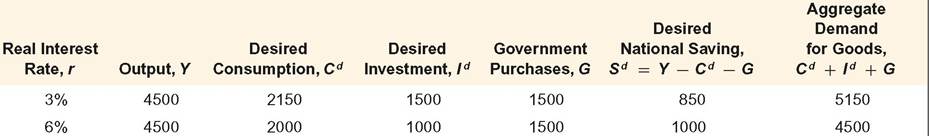
an increase in the real interest rate raises the user cost of capital, which lowers desired investment.

In the example in Table 4.3, when the real interest rate is 6%, desired consump­tion C^d = 2000. Therefore desired national saving S^d = Y — C^d — G = 4500 — 2000 — 1500 = 1000. Also, when the real interest rate is 6%, desired invest­ment I^d = 1000. As desired national saving equals desired investment when r = 6%, the equilibrium real interest rate is 6%, as in Fig. 4.8.

Note, moreover, that when the real interest rate is at the equilibrium value of 6%, the aggregate supply of goods, Y, which is 4500, equals the aggregate demand for goods, C^d + I^d + G = 2000 + 1000 + 1500 = 4500. Thus, both forms of the goods market equilibrium condition, Eqs. (4.7) and (4.8), are satisfied when the real interest rate equals 6%.

Table 4.3 also illustrates how adjustments of the real interest rate bring about equilibrium in the goods market. Suppose that the real interest rate initially is 3%. Both components of private-sector demand for goods (C^d and I^d) are higher when the real interest rate is 3% than when it is 6%. The reason is that consumers save less and firms invest more when real interest rates are relatively low.

Shifts of the Saving Curve. For any real interest rate, a change in the economy that raises desired national saving shifts the saving curve to the right, and a change that reduces desired national saving shifts the saving curve to the left. (Summary table 5 lists the factors affecting desired national saving.)

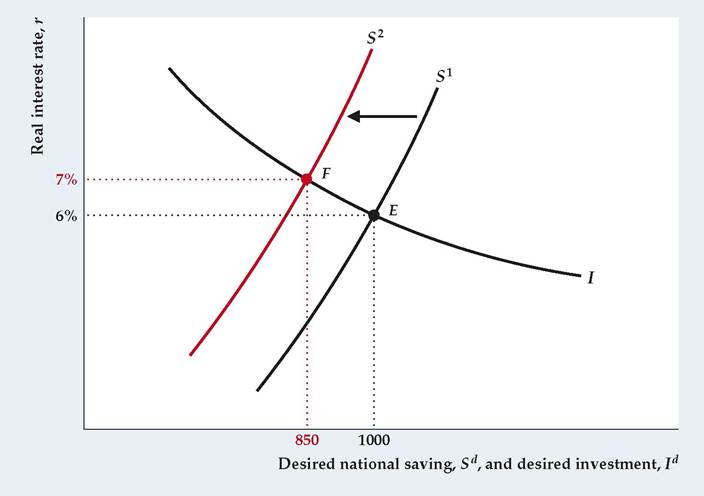
A shift of the saving curve leads to a new goods market equilibrium with a dif­ferent real interest rate and different amounts of saving and investment. Figure 4.9 illustrates the effects of a decrease in desired national saving—resulting, for example, from a temporary increase in current government purchases. The initial equilibrium point is at E, where (as in Fig. 4.8) the real interest rate is 6% and desired national saving and desired investment both equal 1000. When current government pur­chases increase, the resulting decrease in desired national saving causes the saving curve to shift to the left, from S¹ to S². At the new goods market equilibrium point, F, the real interest rate is 7%, reflecting the fact that at the initial real interest rate of 6% the demand for funds by investors now exceeds the supply of saving.

Figure 4.9 also shows that, in response to the increase in government pur­chases, national saving and investment both fall, from 1000 to 850. Saving falls because of the initial decrease in desired saving, which is only partially offset by the increase in the real interest rate. Investment falls because the higher real inter­est rate raises the user cost of capital that firms face. When increased government purchases cause investment to decline, economists say that investment has been crowded out. The crowding out of investment by increased government purchases occurs, in effect, because the government is using more real resources, some of which would otherwise have gone into investment.

FIGURE 4.9

A decline in desired saving

A change that reduces desired national saving, such as a temporary increase in current gov­ernment purchases, shifts the saving curve to the left, from S¹ to S 2. The goods market equilib­rium point moves from E to F. The decline in desired saving raises the real interest rate, from 6% to 7%, and lowers saving and investment, from 1000 to 850.

Shifts of the Investment Curve. Like the saving curve, the investment curve can shift. For any real interest rate, a change in the economy that raises desired investment shifts the investment curve to the right, and a change that lowers desired investment shifts the investment curve to the left. (See Summary table 6 for the factors affecting desired investment.)

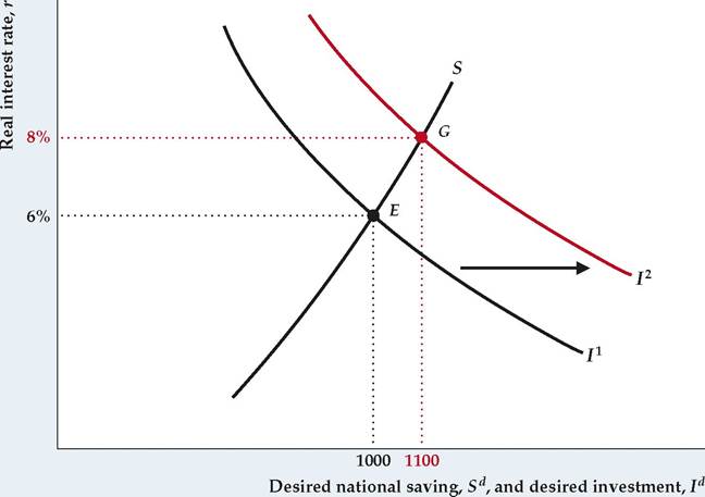
The effects on goods market equilibrium of an increase in desired investment—as from an invention that raises the expected future marginal product of capital—are shown in Figure 4.10. The increase in desired invest­ment shifts the investment curve to the right, from 1¹ to 12, changing the goods market equilibrium point from E to G. The real interest rate rises from 6% to 8% because the increased demand for investment funds causes the real interest rate to be bid up. Saving and investment also increase, from 1000 to 1100, with the higher saving reflecting the willingness of savers to save more when the real interest rate rises.

In these last two chapters, we have presented supply-demand analyses of the labor and goods markets and developed tools needed to understand the behavior of various macroeconomic variables, including employment, the real wage, output, saving, investment, and the real interest rate. These concepts—and a few more developed in the study of asset markets in Chapter 7—form the basis for the economic analysis presented in the rest of this book. In Chapter 5, we use the concepts developed so far to examine the determinants of trade flows and international borrowing and lending. In Chapter 6, we use them to tackle the fundamental question of why some countries' economies grow more quickly than others.

FIGURE 4.10

An increase in desired investment

A change in the economy that increases desired investment, such as an invention that raises the expected future MPK, shifts the investment curve to the right, from 1¹ to 12. The goods market equilibrium point moves from E to G. The real interest rate rises from 6% to 8%, and saving and investment also rise, from 1000 to 1100.

Application

Macroeconomic Consequences of the Boom and Bust in Stock Prices

On October 19, 1987, stock prices took their biggest-ever one-day plunge. The Wilshire 5000 stock price index dropped 18% that day, after having fallen by 15% from the market's peak in August of the same year. About $1 trillion of financial wealth was eliminated by the decline in stock prices on that single day.

Stock prices in the United States soared during the 1990s, especially during the second half of the decade, but then tumbled sharply early in the first year of the new century. Stock prices continued to fall for several years, and stockholders lost wealth of about $5 trillion, an amount equal to about half of a year 's GDP. After rising from 2003 to 2007, stock prices plunged during the financial crisis of

2008, with stocks losing 48% of their value in real terms. By the first quarter of

2009, real stock prices were at their lowest level since 1995. After that, however, stock prices more than tripled from 2009 to 2018.

What are the macroeconomic effects of such booms and busts in stock prices? We have emphasized two major macroeconomic channels for stock prices: a wealth effect on consumption and an effect on capital investment through Tobin's q. Let's see how each of those effects worked after the stock market crash of 1987, the increase in stock values in the 1990s, the decline in stock market wealth in the early 2000s, and the financial crisis of 2008.

The wealth effect on consumption arises because stocks are a component of households' financial assets. Because a stock market boom makes households bet­ter off financially, they should respond by consuming more, and likewise, a bust in

FIGURE 4.11

Real U.S. stock prices and the ratio of consumption to GDP, 1987Q1-2021Q4

The graph shows the val­ues of the real (inflation- adjusted) Wilshire 5000 stock price index, which covers all U.S. corporations with avail­able market prices, and the ratio of consumption spending to GDP from 1987 to the fourth quarter of 2021. The variables move together in some episodes and in opposite directions in other episodes.

Source: Wilshire 5000 index from Wilshire Associates, downloaded from Federal Reserve Bank of St. Louis FRED database at fred.stlouisfed.org∕WILL5000PR; real stock prices calculated as Wilshire 5000 divided by GDP deflator; GDP deflator, consumption spending, and GDP from Bureau of Economic Analysis, downloaded from FRED data­base, series GDPDEF, PCEC, and GDP, respectively.

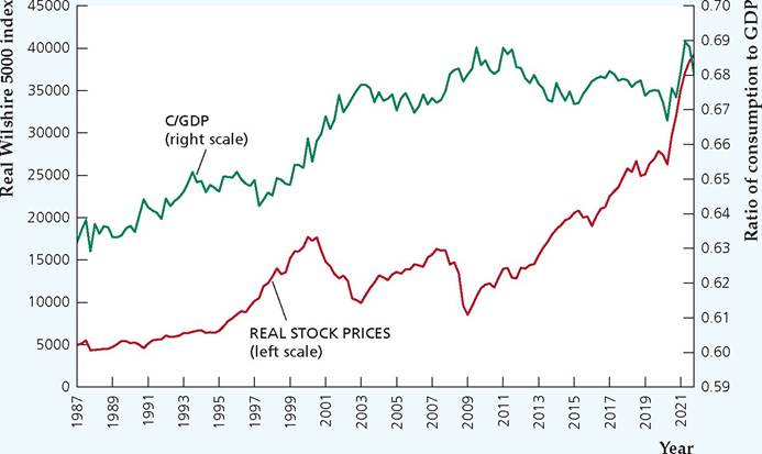
the stock market reduces household wealth and should reduce consumption. To show how consumption and stock prices are related, Figure 4.11 plots the value of the Wilshire 5000 index, adjusted for inflation, along with the ratio of consump­tion spending to GDP.

Consumption and the 1987 Crash

We would expect that following the 1987 stock market crash, consumers would reduce spending, but the decline in consumption should have been much smaller than the $1 trillion decline in wealth because consumers would spread the effects of their losses over a long period of time by reducing planned future consumption as well as current consumption. If consumers spread changes in their wealth over 25 years, then we might guess that current consumption spending would decline by about $40 billion (assuming the real interest rate is near zero). However, consumers might also worry that the stock market crash would lead to a recession, so they might cut consumption further; such a scenario suggests that consumption should decline by more than $40 billion. However, economists who estimated the actual decline in consumption suggest that it fell less than $40 billion.^[68] Why did con­sumption decline less than economic theory suggests? Perhaps the reason is that the rise in stock prices had been very recent—stock prices had risen 39% in the 8 months preceding the crash. Because the increase in stock prices occurred so rap­idly, it is possible that by August 1987, stockholders had not yet fully adjusted their consumption to reflect the higher level of wealth. Thus, when the market fell, con­sumption did not have to decline by very much to fall back into line with wealth.^[69]

Consumption and the Rise in Stock Market Wealth in the 1990s

The U.S. stock market enjoyed tremendous growth during the 1990s. The Wilshire 5000 index more than tripled in real terms by the end of the decade. Our theory predicts that such gains in stock market wealth should be associated with increased consumption spending.

However, contrary to our theory that an increase in wealth should increase consumption, consumption does not appear to have been closely correlated with stock prices in the 1990s. Research by Jonathan Parker shows that there has been a long-run increase in the ratio of consumption to GDP that began in 1979.^[70] He concludes that no more than one-fifth of the increase in the ratio of consumption to GDP in the 1980s and 1990s resulted from increased wealth associated with the stock market boom. And in Fig. 4.11, we can see that stock prices increased signifi­cantly from 1995 to 1998, yet consumption declined relative to GDP in that period.

Consumption and the Decline in Stock Prices in the Early 2000s

Following the peak of the stock market in early 2000, stock prices declined for three years, erasing about $5 trillion in wealth. Our theory suggests that consum­ers should respond by reducing their consumption spending. Yet Fig. 4.11 shows that, in fact, consumption spending increased significantly relative to GDP during that period, rising from 65% of GDP in 1999 to 67% in 2002. Several reasons may explain why consumption did not decline after stock prices fell: (1) the reduction in people's wealth is spread throughout their lifetimes, so there is not a large immediate impact on consumption; (2) at the same time stock prices declined, home prices rose, so many people who lost wealth in the stock market gained it back in real estate; and (3) people may have just viewed their gains in the late 1990s as "paper profits" that were lost in the early 2000s, so neither the gains nor the losses affected consumption.

Investment and the Declines in the Stock Market in the 2000s

As we have seen in Fig. 4.11, the stock market fell precipitously in 2000 and 2008. The large declines in the stock market led to large declines in Tobin's q, the ratio of the market value of firms to the replacement cost of their capital, as you can see in Fig. 4.7 in "In Touch with Data and Research: Investment and the Stock Market." This figure also shows very sharp declines in real investment beginning shortly after the stock market and Tobin's q began to fall in 2000 and again in 2008. The slight delay in the fall in investment, relative to the fall in the stock market, reflects the lags in the process of making investment decisions, planning capital forma­tion, and implementing the plans. But despite these lags, the declines in invest­ment following large declines in the stock market are quite evident.

The Financial Crisis of 2008

During the financial crisis of 2008, stock prices plunged rapidly. In the six months from August 2008 to February 2009, U.S. stock prices declined in nominal terms by 43%, one of the fastest declines in stock prices on record. Investors feared that a depression was possible because of a meltdown in the financial sector, which had taken excessive risks, especially in real-estate markets. The recession that had begun in December 2007 became much worse, and the unemployment rate increased dramatically. In this case, unlike the episode in the early 2000s, home prices also declined, and the simultaneous decline in housing prices and stock values translated into a nearly 20% decline in household net wealth, which fell from $66.7 trillion at the end of 2007 to $55.0 trillion by the end of March 2009. Yet the ratio of consumption to GDP declined by less than 1 percentage point in 2008, as Fig. 4.11 shows, and then it rebounded in early 2009.

The Stock Market Boom Since 2009

After bottoming out in early 2009, the stock market bounced back strongly in the following 12 years, increasing in real terms by more than 300% (from its low point in 2009 to the end of 2021). Consumption spending remained at a high and fairly constant level of about 68% of GDP, but both GDP growth and consumption growth rates were lower than they had been before the financial crisis.

►