Investment
Discuss the
Let s now turn to a second major component of spending: investment spending by factors that aττect firms. Like consumption and saving decisions, the decision about how much to
the investme∩t invest depends largely on expectations about the economy's future.
Investment alsobehavior of firms. shares in common with saving and consumption the idea of a trade-off between the present and the future. In making a capital investment, a firm commits its current resources (which could otherwise be used, for example, to pay increased dividends to shareholders) to increasing its capacity to produce and earn profits in the future.
Recall from Chapter 2 that investment refers to the purchase or construction of capital goods, including buildings, equipment, software, and intellectual property products used in production, and additions to inventory stocks. From a macroeconomic perspective, there are two main reasons to study investment behavior. First, more so than the other components of aggregate spending, investment spending fluctuates sharply over the business cycle, falling in recessions and rising in booms. Even though investment is only about one-sixth of GDP, in the typical recession half or more of the total decline in spending is reduced investment spending. Hence explaining the behavior of investment is important for understanding the business cycle, which we explore further in Part 3.
The second reason for studying investment behavior is that investment plays a crucial role in determining the long-run productive capacity of the economy. Because investment creates new capital goods, a high rate of investment means that the capital stock is growing quickly. As discussed in Chapter 3, capital is one of the two most important factors of production (the other is labor).
All else being equal, output will be higher in an economy that has invested rapidly and thus built up a large capital stock than in an economy that hasn't acquired much capital.The Desired Capital Stock
To understand what determines the amount of investment, we must consider how firms decide how much capital they want. If firms attempt to maximize profit, as we assume, a firm's desired capital stock is the amount of capital that allows the firm to earn the largest expected profit. Managers can determine the profit-maximizing level of the capital stock by comparing the costs and benefits of using additional capital—a new machine, for example. If the benefits outweigh the costs, expanding the capital stock will raise profits. But if the costs outweigh the benefits, the firm
shouldn't increase its planned capital stock and may even want to reduce it. As you might infer from this brief description, the economic logic underlying a firm's decision about how much capital to use is similar to the logic underlying its decision about how many workers to employ, discussed in Chapter 3.
In real terms, the benefit to a firm of having an additional unit of capital is the marginal product of capital, MPK. Recall from Chapter 3 that the MPK is the increase in output that a firm can obtain by adding a unit of capital, holding constant the firm's work force and other factors of production. Because lags occur in obtaining and installing new capital, the expected future marginal product of capital, MPKf, is the benefit from increasing investment today by one unit of capital. This expected future benefit must be compared to the expected cost of using that extra unit of capital, or the user cost of capital.
The User Cost of Capital. To make the discussion of the user cost of capital more concrete, let's consider the case of Kyle's Bakery, Inc., a company that produces specialty cookies. Kyle, the bakery's owner-manager, is considering investing in a new solar-powered oven that will allow him to produce more cookies in the future.
If he decides to buy such an oven, he must also determine its size. In making this decision, Kyle has the following information:1. A new oven can be purchased in any size at a price of $100 per cubic foot, measured in real (base-year) dollars.
2. Because the oven is solar powered, using it does not involve energy costs. The oven also does not require maintenance expenditures.[63] However, the oven becomes less efficient as it ages: With each year that passes, the oven produces 10% fewer cookies. Because of this depreciation, the real value of an oven falls 10% per year. For example, after one year of use, the real value of the oven is $90 per cubic foot.
3. Kyle can borrow (from a bank) or lend (to the government, by buying a one-year government bond) at the prevailing expected real interest rate of 8% per year.
In calculating the user cost of capital, we use the following symbols (the numerical values are from the example of Kyle's Bakery):
pκ = real price of capital goods ($100 per cubic foot); d = rate at which capital depreciates (10% per year); r = expected real interest rate (8% per year).
The user cost of capital is the expected real cost of using a unit of capital for a specified period of time. For Kyle's Bakery, we consider the expected costs of purchasing a new oven, using it for a year, and then selling it. The cost of using the oven has two components: depreciation and interest.
In general, the depreciation cost of using capital is the value lost as the capital wears out. Because of depreciation, after one year the oven for which Kyle pays $100 per cubic foot when new will be worth only $90 per cubic foot. The $10- per-cubic-foot loss that Kyle suffers over the year is the depreciation cost of using the oven. Even if Kyle doesn't sell the oven at the end of a year, he suffers this loss because at the end of the year the asset's (the oven's) economic value will be 10% less.
The interest cost of using capital equals the expected real interest rate times the price of the capital.
As the expected real interest rate is 8% per year, Kyle's interest cost of using the oven for a year is 8% of $100 per cubic foot, or $8 per cubic foot. To see why the interest cost is a cost of using capital, imagine first that Kyle must borrow the funds necessary to buy the oven; in this case, the interest cost of $8 per cubic foot is the interest he pays on the loan, which is obviously part of the total cost of using the oven. Alternatively, if Kyle uses profits from the business to buy the oven, he gives up the opportunity to use those funds to buy an interest-bearing asset, such as a government bond. For every $100 that Kyle puts into the oven, he is sacrificing $8 in interest that he would have earned by purchasing a $100 government bond. This forgone interest is a cost to Kyle of using the oven. Thus the interest cost is part of the true economic cost of using capital, whether the capital's purchase is financed with borrowed funds or with the firm's own retained profits.The user cost of capital is the sum of the depreciation cost and the interest cost. The interest cost is rpK, the depreciation cost is dpK, and the user cost of capital, uc, is
uc = rpκ + dpκ = (r + d)pκ. (4.3)
In the case of Kyle's Bakery,
uc = (0.08 per year ? $100 per cubic foot)
+ (0.10 per year ? $100 per cubic foot)
= $18 per cubic foot per year.
Thus Kyle's user cost of capital is $18 per cubic foot per year.
Determining the Desired Capital Stock. Now we can find a firm's profitmaximizing capital stock, or desired capital stock. A firm's desired capital stock is the capital stock at which the expected future marginal product of capital equals the user cost of capital.
Figure 4.3 shows the determination of the desired capital stock for Kyle's Bakery. The capital stock, K, expressed as cubic feet of oven capacity, is measured along the horizontal axis. Both the MPKf and the user cost of capital are measured along the vertical axis.
The downward-sloping curve shows the value of the MPKf for different sizes of the capital stock, K; at each level of K, the MPKf equals the expected real value of the extra cookies that could be produced per year if oven capacity were expanded an additional cubic foot. The MPKf curve slopes downward because the marginal product of capital falls as the capital stock is increased (we discussed reasons for the diminishing marginal productivity of capital in Chapter 3). The user cost (equal to $18 per cubic foot per year in the example) doesn't depend on the amount of capital and is represented by a horizontal line.
The amount of capital that maximizes the expected profit of Kyle's Bakery is 5000 cubic feet, represented by point A in Fig. 4.3. At A, the expected benefit of an additional unit of capital, MPKf, equals the user cost, uc. For any amount of oven capacity less than 5000 cubic feet, Kyle's Bakery could increase its expected profit by increasing oven capacity. For example, Fig. 4.3 shows that at a planned capacity of 4000 cubic feet the MPKf of an additional cubic foot is $20 worth of cookies per year, which exceeds the $18 per year expected cost of using the additional cubic foot of capacity. Starting from a planned capacity
FIGURE 4.3
Determination of the desired capital stock The desired capital stock (5000 cubic feet of oven capacity in this example) is the capital stock that maximizes profits. When the capital stock is 5000 cubic feet, the expected future marginal product of capital, MPKf, is equal to the user cost of capital, uc. If the MPK f is larger than uc, as it is when the capital stock is 4000 cubic feet, the benefit of extra capital exceeds the cost, and the firm should increase its capital stock. If the MPK f is smaller than uc, as it is at 6000 cubic feet, the cost of extra capital exceeds the benefit, and the firm should reduce its capital stock.
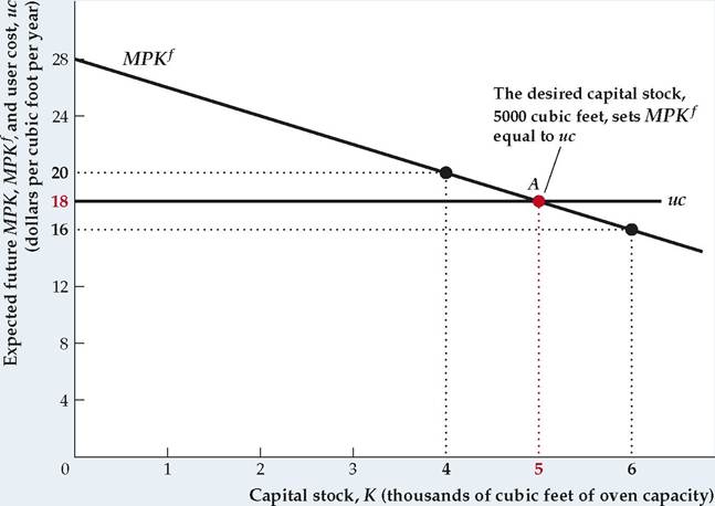
of 4000 cubic feet, if Kyle adds an extra cubic foot of capacity, he will gain an additional $20 worth of future output per year while incurring only $18 per year in expected future costs. Thus expanding beyond 4000 cubic feet is profitable for Kyle. Similarly, Fig. 4.3 shows that at an oven capacity of more than 5000 cubic feet the expected future marginal product of capital, MPKf, is less than the user cost, uc; in this case Kyle's Bakery could increase expected profit by reducing its capital stock. Only when MPKf = uc will the capital stock be at the level that maximizes expected profit.
As mentioned earlier, the determination of the desired capital stock is similar to the determination of the firm's labor demand, described in Chapter 3. Recall that the firm's profit-maximizing level of employment is the level at which the marginal product of labor equals the wage. Analogously, the firm's profit-maximizing level of capital is the level at which the expected future marginal product of capital equals the user cost, which can be thought of as the "wage" of capital (the cost of using capital for one period).
Changes in the Desired Capital Stock
Any factor that shifts the MPKf curve or changes the user cost of capital changes the firm's desired capital stock. For Kyle's Bakery, suppose that the real interest rate falls from 8% per year to 6% per year. If the real interest rate, r, is 0.06 per year and the depreciation rate, d, and the price of capital, pK, remain at 0.10 per year and $100 per cubic foot, respectively, the decline in the real interest rate reduces the user cost of capital, (r + d) pK, from $18 per cubic foot per year to (0.06 + 0.10) $100 per cubic foot per year, or $16 per cubic foot per year.
This decline in the user cost is shown as a downward shift of the user cost line, from uc1 to uc2 in Figure 4.4. After that shift, the MPKf at the original desired capital stock of 5000 cubic feet (point A), or $18 per cubic foot per year,
FIGURE 4.4
A decline in the real interest rate raises the desired capital stock For the Kyle's Bakery example, a decline in the real interest rate from 8% to 6% reduces the user cost, uc, of oven capacity from $18 to $16 per cubic foot per year and shifts the user-cost line down from uc1 to uc2. The desired capital stock rises from 5000 (point A) to 6000 (point C) cubic feet of oven capacity. At 6000 cubic feet the MPKf and the user cost of capital again are equal, at $16 per cubic foot per year.
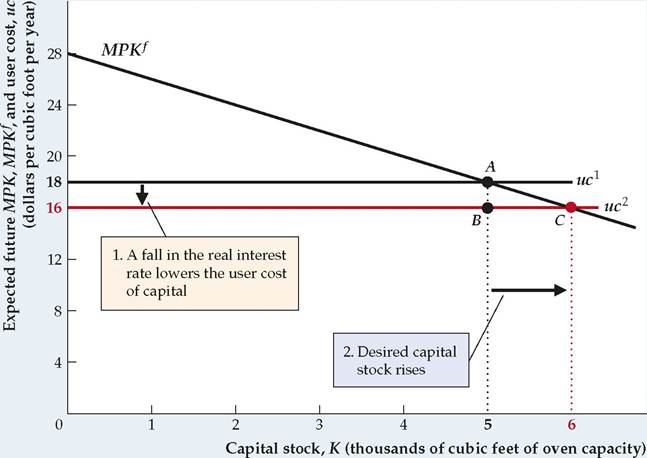
exceeds the user cost of capital, now $16 per cubic foot per year (point B). Kyle's Bakery can increase its profit by raising planned oven capacity to 6000 cubic feet, where the MPKf equals the user cost of $16 per cubic foot per year (point C). This example illustrates that a decrease in the expected real interest rate—or any other change that lowers the user cost of capital—increases the desired capital stock.
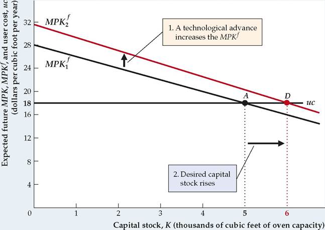
Technological changes that affect the MPKf curve also affect the desired stock of capital. Suppose that Kyle invents a new type of cookie dough that requires less baking time, allowing 12.5% more cookies to be baked daily. Such a technological advance would cause the MPKf curve for ovens to shift upward by 12.5% at each value of the capital stock. Figure 4.5 shows this effect as a shift of the MPKf curve from MPK( to MPK2. If the user cost remains at $18 per cubic foot per year, the technological advance causes Kyle's desired capital stock to rise from 5000 to 6000 cubic feet. At 6000 cubic feet (point D) the MPKf again equals the user cost of capital. In general, with the user cost of capital held constant, an increase in the expected future marginal product of capital at any level of capital raises the desired capital stock.
Taxes and the Desired Capital Stock. So far we have ignored the role of taxes in the investment decision. But Kyle is interested in maximizing the profit his firm gets to keep after paying taxes. Thus he must take into account taxes in evaluating the desirability of an additional unit of capital.
Suppose that Kyle's Bakery pays 20% of its revenues in taxes. In this case, extra oven capacity that increases the firm's future revenues by, say, $20 will raise Kyle's after-tax revenue by only $16, with $4 going to the government. To decide whether to add this extra capacity, Kyle should compare the after-tax MPKf of $16 per cubic foot per year—not the before-tax MPKf of $20 per cubic
FIGURE 4.5
An increase in the expected future MPK raises the desired capital stock
A technological advance raises the expected future marginal product of capital, MPKf, shifting the MPKf curve upward from MPK f to MPK f. The desired capital stock increases from 5000 (point A) to 6000 (point D) cubic feet of oven capacity. At 6000 cubic feet the MPK f equals the user cost of capital uc at $18 per cubic foot per year. firm to subtract a percentage of the purchase price of new capital directly from its tax bill. So, for example, if the investment tax credit is 10%, a firm that purchases a $15,000 piece of equipment can reduce its taxes by $1500 (10% of $15,000) in the year the equipment is purchased.
foot per year—with the user cost. In general, if τ is the tax rate on firm revenues, the after-tax future marginal product of capital is (1 — τ )MPKf. The desired capital stock is the one for which the after-tax future marginal product equals the user cost, or
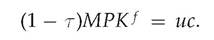
Dividing both sides of this equation by 1 — τ, we obtain
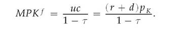 (4.4)
(4.4)
In Eq. (4.4), the term ■ is called the tax-adjusted user cost of capital.
The tax-adjusted user cost of capital shows how large the before-tax future marginal product of capital must be for a firm to willingly add another unit of capital. An increase in the tax rate τ raises the tax-adjusted user cost and thus reduces the desired stock of capital.
To derive the tax-adjusted user cost, we assumed that taxes are levied as a proportion of firms' revenues. However, actual corporate taxes in the United States and other countries are much more complicated. Firms generally pay taxes on their profits rather than on their revenues, and the part of profit that is considered taxable may depend on how much the firm invests. For example, when a firm purchases some capital, it is allowed to deduct part of the purchase price of the capital from its taxable profit in both the year of purchase and in subsequent years. By reducing the amount of profit to be taxed, these deductions, known as depreciation allowances, allow the firm to reduce its total tax payment.
Another important tax provision, which has been used at various times in the United States, is the investment tax credit. An investment tax credit permits the
Economists summarize the many provisions of the tax code affecting investment by a single measure of the tax burden on capital called the effective tax rate. Essentially, the idea is to ask: What tax rate τ on a firm's revenue would have the same effect on the desired capital stock as do the actual provisions of the tax code? The hypothetical tax rate that answers this question is the effective tax rate. Changes in the tax law that, for example, raise the effective tax rate are equivalent
Application To get around the problem that factors other than taxes are always changing, Cummins, Hubbard, and Hassett focused on the periods around 13 major tax reforms, beginning with the investment tax credit initiated by President John F. Kennedy in 1962 and ending with the major tax reform of 1986, passed under President Ronald Reagan. The authors' idea was that, by looking at occasions when the tax code changed significantly in a short period of time, they could reasonably assume that most of the ensuing change in investment was the result of the tax change rather than other factors. To get around the second problem, that tax cuts tend to take place when aggregate investment is low, Cummins, Hubbard, and Hassett didn't look at the behavior of aggregate investment; instead, they compared the investment responses of a large number of individual corporations to each tax reform. Because the tax laws treat different types of capital differently (for example, a machine and a factory are taxed differently) and because companies use capital in different combinations, the authors argued that observing how different companies changed their investment after each tax reform would provide information on the effects of the tax changes. For example, if a tax reform cuts taxes on machines relative to taxes on factories and taxes are an important determinant of investment, companies whose investment is concentrated in machinery should respond relatively more strongly to the tax change than companies who invest primarily in factories.
Cummins, Hubbard, and Hassett found considerably stronger effects of tax changes on investment than reported in previous studies, possibly because the earlier studies didn't deal effectively with the two problems that we identified. These authors found an empirical elasticity of about — 0.66. That is, according to their estimates, a tax change that lowers the user cost of capital by 10% would raise aggregate investment by about 6.6%, a significant amount. Thus, the effective tax rate significantly affects investment.
TABLE 4.2
Effective Tax Rate on Capital, 2019
| ETR | IIGDP | ETR | IIGDP | ||
| Australia | 14.9 | 22.3 | Japan | 23.4 | 25.5 |
| Austria | 16.7 | 25.4 | Korea (Rep. of) | 13.7 | 30.1 |
| Belgium | -19.1 | 25.2 | Luxembourg | 11.9 | 18.0 |
| Canada | 7.1 | 21.9 | Mexico | 15.7 | 19.9 |
| Chile | 23.9 | 22.2 | Netherlands | 14.2 | 22.3 |
| Czech Republic | 10.3 | 28.1 | New Zealand | 23.5 | 24.9 |
| Denmark | 8.4 | 21.8 | Norway | 10.3 | 29.8 |
| Finland | 16.3 | 23.0 | Poland | -5.8 | 20.2 |
| France | 9.9 | 24.3 | Portugal | -24.8 | 18.0 |
| Germany | 16.9 | 21.3 | Slovak Republic | 8.6 | 24.0 |
| Greece | 15.3 | 12.3 | Slovenia | 7.9 | 20.3 |
| Hungary | 4.7 | 27.6 | Spain | 11.8 | 20.6 |
| Iceland | 12.5 | 21.1 | Sweden | 13.1 | 24.9 |
| Ireland | 10.5 | 54.7 | Switzerland | 12.1 | 24.7 |
| Israel | 12.1 | 22.3 | Turkey | -5 | 0.0 |
| Italy | -42.4 | 18.3 | United Kingdom | 3.7 | 17.9 |
| United States | -2.7 | 21.9 |
Note: ETR is effective tax rate on capital in 2019, in percent. I/GDP is the ratio of gross capital formation to GDP in percent, for 2019.
Sources: ETR from OECD.Stat, https://stats.oecd.org/index.aspx?DataSetCode=CTS_ETR I/GDPfrom OECD. Stat, https://stats.oecd.org/index.aspx?DataSetCode=SNA_TABLE1 variables P5: gross capital formation and B1 GA: GDP (output approach)
From the Desired Capital Stock to Investment
Now let's look at the link between a firm's desired capital stock and the amount it invests. In general, the capital stock (of a firm or of a country) changes over time through two opposing channels. First, the purchase or construction of new capital goods increases the capital stock. We've been calling the total purchase or construction of new capital goods that takes place each year "investment," but its precise name is gross investment. Second, the capital stock depreciates or wears out, which reduces the capital stock.
Whether the capital stock increases or decreases over the course of a year depends on whether gross investment is greater or less than depreciation during the year; when gross investment exceeds depreciation, the capital stock grows. The change in the capital stock over the year—or, equivalently, the difference between gross investment and depreciation—is net investment.
We express these concepts symbolically as
It = gross investment during year t,
Kt = capital stock at the beginning of year t, and
Kt+1 = capital stock at the beginning of year t + 1
(equivalently, at the end of year t).
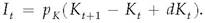
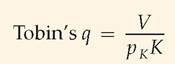
Net investment, the change in the capital stock during period t, equals Kt+1 — Kt. The amount of depreciation during year t is dKt, where d is the fraction of capital that depreciates each year. The relationship between net and gross investment is
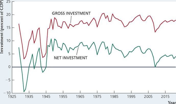
In most but not all years, gross investment is larger than depreciation so that net investment is positive and the capital stock increases. Figure 4.6 shows the behavior since 1929 of gross and net investment in the United States, expressed as percentages of GDP; the difference between gross and net investment is depreciation. Note the occasional large swings in both gross and net investment and the negative rates of net investment that occurred in some years during the Great Depression of the 1930s and World War II (1941-1945). Net investment was very low from 2009 to 2011 in the aftermath of the financial crisis.
We use Eq. (4.5) to illustrate the relationship between the desired capital stock and investment. First, rewriting Eq. (4.5) gives
which states that gross investment equals net investment plus depreciation.[64]
Now suppose that firms use information available at the beginning of year t about the expected future marginal product of capital and the user cost of capital and determine the desired capital stock, K*, they want by the end of year t (the beginning of year t + 1). For the moment, suppose also that capital is easily
FIGURE 4.6
Gross and net investment, 1929-2021 Gross and net investment in the United States since 1929 are shown as percentages of GDP. During some years of the Great Depression and World War II net investment was negative, implying that the capital stock was shrinking.
Sources: GDP, gross private domestic investment, and net private domestic investment from Bureau of Economic Analysis, downloaded from Federal Reserve Bank of St. Louis FRED database, fred.stlouisfed.org, series GDPA, GPDIA, and A557RC1A027NBEA.
obtainable so that firms can match the actual capital stock at the end of year t, Kt+1, with the desired capital stock, K *. Substituting K * for Kt+1 in the preceding equation yields

Equation (4.6) shows that firms' gross investment, It, during a year has two parts: (1) the desired net increase in the capital stock over the year, K * — Kt; and (2) the investment needed to replace worn-out or depreciated capital, dKt. The amount of depreciation that occurs during a year is determined by the depreciation rate and the initial capital stock. However, the desired net increase in the capital stock over the year depends on the factors—such as taxes, interest rates, and the expected future marginal product of capital—that affect the desired capital stock. Indeed, Eq. (4.6) shows that any factor that leads to a change in the desired capital stock, K *, results in an equal change in gross investment, It.
Lags and Investment. The assumption just made—that firms can obtain capital quickly enough to match actual capital stocks with desired levels each year—isn't realistic in all cases. Although most types of equipment are readily available, a skyscraper or a nuclear power plant may take years to construct. Thus, in practice, a $1 million increase in a firm's desired capital stock may not translate into a $1 million increase in gross investment within the year; instead, the extra investment may be spread over several years as planning and construction proceed. Despite this qualification, factors that increase firms' desired capital stocks also tend to increase the current rate of investment. Summary table 6 brings together the factors that affect investment. In "In Touch with Data and Research: Investment and the Stock Market," we discuss an alternative approach to investment, which relates investment to stock prices.
Investment in Inventories and Housing
Our discussion so far has emphasized what is called business fixed investment, or investment by firms in structures (such as factories and office buildings), equipment (such as drill presses and jetliners), software, and intellectual property. However, there are two other components of investment spending: inventory investment and residential investment. As discussed in Chapter 2, inventory investment equals the increase in firms' inventories of unsold goods, unfinished goods, or raw materials. Residential investment is the construction of housing, such as single-family homes, condominiums, or apartment buildings.
| SUMMARY 6 | ||
| Determinants of Desired Investment | ||
| An increase in | Causes desired investment to | Reason |
| Real interest rate, r | Fall | The user cost increases, which reduces desired capital stock. |
| Effective tax rate, τ | Fall | The tax-adjusted user cost increases, which reduces desired capital stock. |
| Expected future MPK | Rise | The desired capital stock increases. |
Fortunately, the concepts of future marginal product and the user cost of capital, which we used to examine business fixed investment, apply equally well to inventory investment and residential investment. Consider, for example, Patricia, a new-car dealer trying to decide whether to increase the number of cars she normally keeps on her lot from 100 to 150—that is, whether to make an inventory investment of 50 cars. The benefit of having more cars to show is that potential car buyers will have a greater variety of models from which to select and may not have to wait for delivery, enabling the car dealer to sell more cars. The increase in sales commissions the car dealer expects to make, measured in real terms and with the same sales force, is the expected future marginal product of the increased inventory. The cost of holding more cars reflects (1) depreciation of the cars sitting on the lot and (2) the interest the car dealer must pay on the loan obtained to finance the higher inventory. The car dealer will make the inventory investment if the expected benefits of increasing her inventory, in terms of increased sales commissions, are at least as great as the interest and depreciation costs of adding 50 cars. This principle is the same one that applies to business fixed investment.
In Touch with Data and Research
Investment and the Stock Market
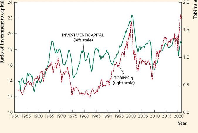
Fluctuations in the stock market can have important macroeconomic effects. Changes in stock prices may cause households to change how much they consume and save (see the Application "Macroeconomic Consequences of the Boom and Bust in Stock Prices"). Similarly, economic theory suggests that rises and falls in the stock market should lead firms to change their rates of capital investment in the same direction. The relationship between stock prices and firms' investment in physical capital is captured by the "q theory of investment," developed by James Tobin, who was a Nobel laureate at Yale University.
Tobin argued that the rate of investment in any particular type of capital can be predicted by looking at the ratio of the capital's market value to its replacement cost. When this ratio, often called "Tobin's q," is greater than 1, it is profitable to acquire additional capital because the value of capital exceeds the cost of acquiring it. Similarly, when Tobin's q is smaller than 1, the value of capital is less than the cost of acquiring it, so it is not profitable to invest in additional capital.[65]
Because much of the value of firms comes from the capital they own, we can use the stock market value of a firm as a measure of the market value of the firm's capital stock. If we let V be the stock market value of a firm, K be the amount of capital the firm owns, and pκ be the price of new capital goods, then for an individual firm
where pκK is the replacement cost of the firm's capital stock. If the replacement cost of capital isn't changing much, a boom in the stock market (an increase in V)
FIGURE 4.7
Ratio of Investment to Capital and Tobin's q, 1951Q4-2021Q3
The graph shows the ratio of investment to the capital stock on the left axis and the value of Tobin's q on the right axis. Note that the invest- ment/capital ratio and Tobin's q usually move together, rising or falling at about the same time.
Source: Investment is nonfinan- cial fixed investment from Bureau of Economic Analysis, downloaded from St. Louis Fed website at fred.stlouisfed.org series PNFI; capital is sum of nonfi- nancial corporate sector equipment and structures, FRED series Rcsnnwmvbsnncb and ESABSNNCB; Tobin's q is the ratio of nonfinancial corporate sector equities value, FRED series Mveonwmvbsnncb, to net worth, FRED series tnwmvbsnncb.
will cause Tobin's q to rise for most firms, leading to increased rates of investment. Essentially, when the stock market is high, firms find it profitable to expand.
Figure 4.7 shows quarterly data on Tobin's q and the ratio of investment to capital. Consistent with the theory, the two are closely related; Tobin's q and investment rose together in the 1950s, 1960s, and 2010s, and then both fell sharply in 2000 and 2008. However, from 1975 to 1995, Tobin's q and the ratio of investment to capital are less closely related.
Although it may seem different, the q theory of investment is similar to the theory of investment discussed in this chapter. In the theory developed in this chapter we identified three main factors affecting the desired capital stock: the expected future marginal product of capital, MPKf; the real interest rate, r; and the purchase price of new capital, pκ. Each of these factors also affects Tobin's q: (1) An increase in the expected marginal product of capital tends to increase the expected future earnings of the firm, which raises the stock market value of the firm and thus increases q; (2) a reduction in the real interest rate also tends to raise stock prices (and hence q), as financial investors substitute away from low-yielding bonds and bank deposits and buy stocks instead; and (3) a decrease in the purchase price of capital reduces the denominator of the q ratio and thus increases q. Because all three types of change increase Tobin's q, they also increase the desired capital stock and investment, as predicted by our analysis in this chapter.
4.3
More on the topic Investment:
- Malta
- Qatar
- Recent developments
- Background Context
- Introduction
- FINAL WORDS
- Engines of Empire: The Chartered, Limited Liability Joint Stock Companies
- The Netherlands and the UK: The Witteveen Reports and their contradictory results
- 2 Husbandry and estate management: statutory standards
- Statement—Courses of Action