Consumption and Saving
Discuss the
We begin consideration of the demand for goods and services by discussing the fac- τactors that aττect tors that affect consumer spending.
Because consumption spending by households iscθ∏su∣τ∣ption and by far the largest component of the demand for goods and services—accounting for
saving decisions. more than two-thirds of total spending in the United States—changes in consumers' willingness to spend have major implications for the behavior of the economy.
Besides the sheer size of consumption spending, another reason to study consumption is that the individual's or household's decision about how much to consume is closely linked to another important economic decision, the decision about how much to save. Indeed, for given levels of disposable income, the decision about how much to consume and the decision about how much to save are really the same decision. For example, Evelyn Yamaguchi, a college student with a parttime job that pays $8000 per year after taxes might decide to spend $7400 per year on clothes, food, entertainment, and other consumption. If she does consume this amount, her saving will automatically be $600 ($8000 minus $7400) per year. Equivalently, she might decide to save $600 per year. If she succeeds in saving $600, her consumption automatically is $7400 ($8000 minus $600) per year. Because the decision about how much to consume and the decision about how much to save actually are two sides of the same coin, we analyze them together.
From a macroeconomic perspective, we are interested in the aggregate, or national, levels of consumption and saving. We define the national level of desired consumption, Cd, as the aggregate quantity of goods and services that households want to consume, given income and other factors that determine households' economic opportunities.
We will analyze desired consumption and its response to various factors, such as income and interest rates, by examining the consumption decisions of individual households. The aggregate level of desired consumption, Cd, is obtained by adding up the desired consumption of all households. Thus any factor that increases the desired consumption of individual households will increase Cd, and any factor that decreases the desired consumption of individual households will decrease Cd.Just as a household's consumption decision and saving decision are closely linked, a country's desired consumption is closely linked to its desired national saving. Specifically, desired national saving, Sd, is the level of national saving that occurs when aggregate consumption is at its desired level.[LIV] Recall from Chapter 2 (Eq. 2.8) that if net factor payments from abroad (NFP) equal zero (as must be true in a closed economy), national saving, S, equals Y — C — G, where Y is output, C is consumption, and G is government purchases. Because desired national saving, Sd, is the level of national saving that occurs when consumption equals its desired level, we obtain an expression for desired national saving by substituting desired consumption, Cd, for consumption, C, in the definition of national saving. This substitution yields

We can gain insight into the factors that affect consumption and saving at the national level by considering how consumption and saving decisions are made at the individual level. Appendix 4.A provides a more formal analysis of this decision-making process.
The Consumption and Saving Decision of an Individual
Let's consider the case of Prudence, a bookkeeper for the Spectacular Eyeglasses Company. Prudence earns $60,000 per year after taxes. Hence she could, if she chose, consume $60,000 worth of goods and services every year.
Prudence, however, has two other options.First, she can save by consuming less than $60,000 per year. Why should Prudence consume less than her income allows? The reason is that she is thinking about the future. By consuming less than her current income, she will accumulate savings that will allow her, at some time in the future, to consume more than her income. For example, Prudence may expect her income to be very low when she retires; by saving during her working life, she will be able to consume more than her income during retirement. Indeed, the desire to provide for retirement is an important motivation for saving in the real world.
Alternatively, Prudence could consume more than her current income by borrowing or by drawing down previously accumulated savings. If she borrows $5000 from a bank, for example, she could consume as much as $65,000 worth of goods and services this year even though her income is only $60,000. Consuming more than her income is enjoyable for Prudence, but the cost to her is that at some future time, when she must repay the loan, she will have to consume less than her income.
If Prudence consumes less today, she will be able to consume more in the future, and vice versa. In other words, she faces a trade-off between current consumption and future consumption. The rate at which Prudence trades off current and future consumption depends on the real interest rate prevailing in the economy. Suppose that Prudence can earn a real interest rate of r per year on her saving and, for simplicity, suppose that if she borrows, she must pay the same real interest rate r on the loan. These assumptions imply that Prudence can trade one unit of
current (this year's) consumption for 1 + r units of future (next year's) consumption. For example, suppose Prudence reduces her consumption today by one dollar, thereby increasing her saving by one dollar. Because she earns a real interest rate of r on her saving, the dollar she saves today will be worth 1 + r dollars one year from now.[LV] Under the assumption that Prudence uses the extra 1 + r dollars to increase her next year 's consumption, she has effectively traded one dollar's worth of consumption today for 1 + r dollars of consumption a year from now.
Similarly, Prudence can trade 1 + r real dollars of future consumption for one extra dollar of consumption today. She does so by borrowing and spending an extra dollar today. In a year she will have to repay the loan with interest, a total of 1 + r dollars. Because she has to repay 1 + r dollars next year, her consumption next year will be 1 + r dollars less than it would be otherwise. So the "price" to Prudence of one dollar's worth of extra consumption today is 1 + r dollars' worth of consumption in the future.
The real interest rate r determines the relative price of current consumption and future consumption. Given this relative price, how should Prudence choose between consuming today and consuming in the future? One extreme possibility would be for her to borrow heavily and consume much more than her income today. The problem with this strategy is that, after repaying her loan, Prudence would be able to consume almost nothing in the future. The opposite, but equally extreme, approach would be for Prudence to save nearly all of her current income. This strategy would allow her to consume a great deal in the future, but at the cost of near-starvation today.
Realistically, most people would choose neither of those extreme strategies but would instead try to avoid sharp fluctuations in consumption. The desire to have a relatively even pattern of consumption over time—avoiding periods of very high or very low consumption—is known as the consumption-smoothing motive. Because of her consumption-smoothing motive, Prudence will try to spread her consumption spending more or less evenly over time, rather than bingeing in one period and starving in another.
Next, we will see how the consumption-smoothing motive guides Prudence's behavior when changes occur in some important determinants of her economic well-being, including her current income, her expected future income, and her wealth. As we consider each of these changes, we will hold constant the real interest rate r and, hence, the relative price of current consumption and future consumption.
Later, we will discuss what happens if the real interest rate changes.Effect of Changes in Current Income
Current income is an important factor affecting consumption and saving decisions. To illustrate, suppose that Prudence receives a one-time bonus of $6000 at work, which increases her current year's income by $6000. (We ignore income taxes; equivalently, we can assume that the bonus is actually larger than $6000 but that, after paying her taxes, Prudence finds that her current income has increased by $6000.) What will she do with this extra income? Prudence could splurge and spend the entire bonus on a trip to Hawaii. If she spends the entire bonus, her current consumption will increase by $6000, but because she has not increased her saving, her future consumption will be unchanged. Alternatively, she could save the entire bonus, leaving her current consumption unchanged but using the bonus plus the interest it earns to increase her consumption in the future. Because of the consumption-smoothing motive, however, Prudence is unlikely to follow either of these extreme strategies. Instead, she will spend part of the bonus (increasing current consumption) and save the rest (enabling her to increase future consumption as well).
The portion of her bonus that Prudence spends will depend on factors such as her willingness to defer gratification and her assessment of her current and future needs. We define Prudence's marginal propensity to consume (MPC) as the fraction of additional current income that she consumes in the current period. Because Prudence consumes some but not all of her extra income, her MPC will be between zero and one. Suppose, for example that Prudence has an MPC equal to 0.4, so that she consumes 0.4, or 40%, of an increase in current income. Then, when she receives a $6000 bonus, Prudence will increase her current consumption by 0.4 ? $6000 = $2400. Because the part of income that is not consumed is saved, her saving also increases by the amount of $6000 — $2400 = $3600.
The marginal propensity to consume also applies to declines in current income. For example, if Prudence were temporarily laid off from her bookkeeping job so that her current year's income decreased by $8000, she would reduce both her consumption and her saving. If we assume that her marginal propensity to consume remains 0.4, she would reduce her consumption by 0.4 ? $8000 = $3200, and her saving would therefore have to diminish by $8000 — $3200 = $4800.
Aggregate income and consumption reflect the decisions of millions of individuals and households, so that the lessons we learned from thinking about the case of Prudence also apply at the macroeconomic level. Just as an increase in Prudence's income caused her to consume more, we would expect an increase in aggregate output (income) Y to lead to an increase in aggregate desired consumption, Cd, as well. Because marginal propensities to consume are less than 1, however, the increase in Cd will be less than the increase in Y. As not all of the increase in Y is spent, desired national saving Sd will also rise when Y rises.
Effect of Changes in Expected Future Income
Today's consumption decisions may depend not only on current income but also on the income that one expects to earn in the future. For example, an individual who is currently not employed but who has a contract to begin a high-paying job in three months will probably consume more today than a similar individual who is currently not employed but has no prospects for a job in the near future.
To illustrate the effect of changes in expected future income, suppose that instead of receiving the $6000 bonus during the current year, Prudence learns that she will receive a $6000 bonus (after taxes) next year. The promise of the bonus is legally binding, and Prudence has no doubt that she will receive the extra income next year. How will this information affect Prudence's consumption and saving in the current year?
Because her current income is unaffected, Prudence could leave her current consumption and saving unchanged, waiting until she actually receives the bonus to increase her consumption. If her decisions are guided by a consumption-smoothing motive, however, she will prefer to use the bonus to increase her current consumption as well as her future consumption. She can increase her current consumption, despite the fact that her current income remains unchanged, by reducing her current saving (she could even "dissave," or have negative current saving, with current consumption exceeding current income, by using her accumulated assets or by borrowing). Suppose, for example, that Prudence decides to consume $1000 more this year. Because her current income is unchanged, Prudence's $1000 increase in current consumption is equivalent to a $1000 reduction in current saving.
The $1000 reduction in current saving will reduce Prudence's available resources in the next year, relative to the situation in which her saving is unchanged, by $1000 ? (1 + r). For example, if the real interest rate is 0.05 per year, cutting current saving by $1000 reduces Prudence's available resources next year by $1000 ? 1.05 = $1050. Overall, her available resources next year will increase by $6000 because of the bonus but will decrease by $1050 because of reduced current saving, giving a net increase in resources of $6000 — $1050 = $4950, which can be used to increase consumption next year or in the following years. Effectively, Prudence can use the increase in her expected future income to increase consumption both in the present and in the future.
To summarize, an increase in an individual's expected future income is likely to lead that person to increase current consumption and decrease current saving. The same result applies at the macroeconomic level: If people expect that aggregate output and income, Y, will be higher in the future, current desired consumption, Cd, should increase and current desired national saving, Sd, should decrease. Consumption and saving can also be affected by other shocks, as we discuss in the Application "The Impact of the Pandemic Recession of 2020 on Consumption."
Application
The Impact of the Pandemic Recession of 2020 on Consumption
In March 2020, a global pandemic affected the world's economies in significant ways. Governments throughout the world shut down portions of their economies so that people would not come in close contact with each other until a vaccine could be developed. The result was a sharp decline in economic activity that caused a deep recession, much deeper than any recession since the Great Depression in the 1930s and far worse than in the Global Financial Crisis in 2008, as Figure 4.1
FIGURE 4.1
Real GDP Growth Rate, 1980Q1-2021Q4 The quarterly, annualized growth rate of real GDP had its biggest decline in history in the second quarter of 2020 followed by the largest increase in history in the third quarter of 2020. The pandemic recession of 2020 was the shortest recession in history as well.
Source: FRED database, Federal Reserve Bank of St. Louis, fred.stlouisfed.org/series/GDPC1.
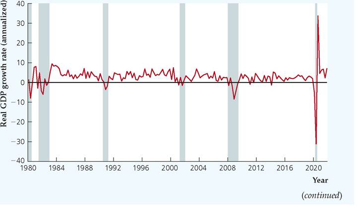
FIGURE 4.2
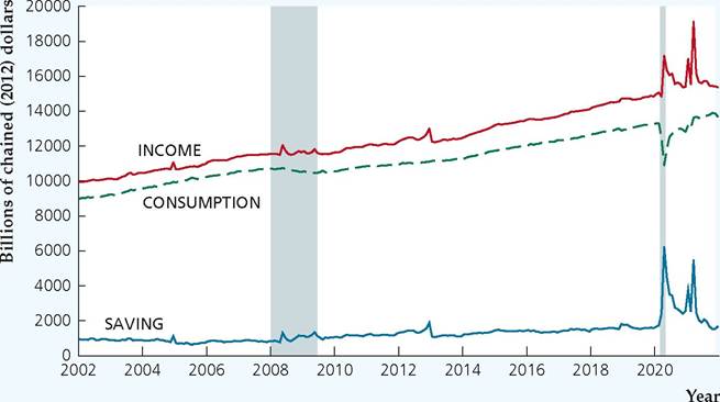
Income, Consumption, and Saving, January 2002-December 2021
Monthly income, consumption, and saving showed dramatic changes during and following the pandemic recession. Income spiked up because of government programs, while consumption declined because people avoided contact with each other. As a result, saving rose substantially for more than a year.
Source: FRED database, Federal Reserve Bank of St. Louis, fred.stlouisfed.org. Income is real disposable personal income, series DSPIC96. Consumption is real personal consumption expenditures, series PCEC96. Saving is income minus consumption.
illustrates. However, because of its unusual source, the recession was also the shortest in history, lasting only two months.
The sudden drop in income for many people led governments to provide support to help replace lost incomes. For example, in the United States, the Federal government greatly increased the unemployment insurance program and sent cash directly to many people whose incomes were below a certain level, in addition to other programs. As a result, the level of after-tax disposable income actually increased, rather than declining, during the recession and for some time after it was over. Nonetheless, overall consumer spending declined sharply, as people avoided spending activities that involved direct contact, especially on travel and dining. The increase in incomes and decline in consumer spending led to an increase in saving, as Figure 4.2 shows.
People's spending patterns also changed. Because of the need to avoid close contact with other people, spending on entertainment services, travel, and dining all dropped sharply. People spent more of their incomes on purchases of goods rather than services. This change in patterns of consumer spending then led to changes in the demand for workers in the different sectors. It remains to be seen whether these changes in the demand for goods and workers will be temporary or permanent.
Effect of Changes in Wealth
Another factor that affects consumption and saving is wealth. Recall from Chapter 2 that the wealth of any entity, such as a household or an entire nation, equals its assets minus its liabilities.
To see how consumption and saving respond to an increase in wealth, suppose that while organizing her father's finances Prudence finds a stock certificate for 50 shares of stock in a pharmaceutical company. Prudence's grandmother bought this stock for Prudence when she was born, and Prudence did not know about it. She immediately calls her broker and learns that the stock is now worth $6000. This unexpected $6000 increase in Prudence's wealth has the same effect on her available resources as the $6000 increase in current income that we examined earlier. As in the case involving an increase in her current income, Prudence will use her increase in wealth to increase her current consumption by an amount smaller than $6000 so that she can use some of the additional $6000 to increase her future consumption. Because Prudence's current income is not affected by finding the stock certificate, the increase in her current consumption is matched by a decrease in current saving of the same size. In this way, an increase in wealth increases current consumption and reduces current saving. The same line of reasoning leads to the conclusion that a decrease in wealth reduces current consumption and increases saving.
The ups and downs in the stock market are an important source of changes in wealth, and the effects on consumption of changes in the stock market are explored in the Application "Macroeconomic Consequences of the Boom and Bust in Stock Prices."
Effect of Changes in the Real Interest Rate
We have seen that the real interest rate is the price of current consumption in terms of future consumption. We held the real interest rate fixed when we examined the effects of changes in current income, expected future income, and wealth. Now we let the real interest rate vary, examining the effect of changes in the real interest rate on current consumption and saving.
How would Prudence's consumption and saving change in response to an increase in the real interest rate? Her response to such an increase reflects two opposing tendencies. On the one hand, because each real dollar of saving in the current year grows to 1 + r real dollars next year, an increase in the real interest rate means that each dollar of current saving will have a higher payoff in terms of increased future consumption. This increased reward for current saving tends to increase saving.
On the other hand, a higher real interest rate means that Prudence can achieve any future savings target with a smaller amount of current saving. For example, suppose that she is trying to accumulate $1400 to buy a new laptop computer next year. An increase in the real interest rate means that any current saving will grow to a larger amount by next year, so the amount that she needs to save this year to reach her goal of $1400 is lower. Because she needs to save less to reach her goal, she can increase her current consumption and thus reduce her saving.
The two opposing effects described above are known as the substitution effect and the income effect of an increase in the real interest rate. The substitution effect of the real interest rate on saving reflects the tendency to reduce current consumption and increase future consumption as the price of current consumption, 1 + r, increases. In response to an increase in the price of current consumption, consumers substitute away from current consumption, which has become relatively more expensive, toward future consumption, which has become relatively less expensive. The reduction in current consumption implies that current saving increases. Thus the substitution effect implies that current saving increases in response to an increase in the real interest rate.
The income effect of the real interest rate on saving reflects the change in current consumption that results when a higher real interest rate makes a consumer richer or poorer. For example, if Prudence has a savings account and has not borrowed any funds, she is a recipient of interest payments. She therefore benefits from an increase in the real interest rate because her interest income increases. With a higher interest rate, she can afford to have the same levels of current and future consumption as before the interest rate change, and she would have some additional resources to spend. These extra resources are effectively the same as an increase in her wealth, so she will increase both her current and her future consumption. Thus, for a saver, who is a recipient of interest payments, the income effect of an increase in the real interest rate is to increase current consumption and reduce current saving. Therefore, for a saver, the income and substitution effects of an increase in the real interest rate work in opposite directions, with the income effect reducing saving and the substitution effect increasing saving.
The income effect of an increase in the real interest rate is different for a payer of interest, such as a borrower. An increase in the real interest rate increases the amount of interest payments that a borrower must make, thereby making the borrower unable to afford the same levels of current and future consumption as before the increase in the real interest rate. The borrower has effectively suffered a loss of wealth as a result of the increase in the real interest rate and responds to this decline in wealth by reducing both current consumption and future consumption. The reduction in current consumption means that current saving increases (that is, borrowing decreases). Hence, for a borrower, the income effect of an increase in the real interest rate is to increase saving. Thus both the substitution effect and the income effect of an increase in the real interest rate increase the saving of a borrower.
Let's summarize the effect of an increase in the real interest rate. For a saver, who is a recipient of interest, an increase in the real interest rate tends to increase saving through the substitution effect but to reduce saving through the income effect. Without additional information, we cannot say which of these two opposing effects is larger. For a borrower, who is a payer of interest, both the substitution effect and the income effect operate to increase saving. Consequently, the saving of a borrower unambiguously increases.
What is the effect of an increase in the real interest rate on national saving? Because the national economy is composed of both borrowers and savers, and because, in principle, savers could either increase or decrease their saving in response to an increase in the real interest rate, economic theory cannot answer this question. Because economic theory does not indicate whether national saving increases or decreases in response to an increase in the real interest rate, we must rely on empirical studies that examine this relationship using actual data. Unfortunately, interpretation of the empirical evidence from the many studies done continues to inspire debate. The most widely accepted conclusion seems to be that an increase in the real interest rate reduces current consumption and increases saving, but this effect isn't very strong.
Taxes and the Real Return to Saving. In discussing the real return that savers earn, we have not yet mentioned an important practical consideration: Interest earnings (and other returns on savings) are taxed. Because part of interest earnings must be paid as taxes, the real return earned by savers is actually less than the difference between the nominal interest rate and expected inflation.
A useful measure of the returns received by savers that recognizes the effects of taxes is the expected real after-tax interest rate. To define this concept, we let i represent the nominal interest rate and t the rate at which interest income is taxed. In the United States, for example, most interest earnings are taxed as ordinary income, so t is the income tax rate. Savers retain a fraction (1 — t) of total interest
earned so that the nominal after-tax interest rate, received by savers after payment of taxes, is The expected real after-tax interest rate, ra_t, is the after-tax
nominal interest rate minus the expected inflation rate, πe, or

The expected real after-tax interest rate is the appropriate interest rate for consumers to use in making consumption and saving decisions because it measures the increase in the purchasing power of their saving after payment of taxes.
Table 4.1 shows how to calculate the nominal after-tax interest rate and the expected real after-tax interest rate. Note that, given the nominal interest rate and expected inflation, a reduction in the tax rate on interest income increases the nominal and real after-tax rates of return that a saver receives. Thus, by reducing the rate at which it taxes interest, the government can increase the real rate of return earned by savers and (possibly) increase the rate of saving in the economy.
The stimulation of saving is the motivation for tax provisions, such as individual retirement accounts (IRAs), that allow savers to shelter part of their interest earnings from taxes and thus earn higher after-tax rates of return. Unfortunately, because economists disagree about the effect of higher real interest rates on saving, the effectiveness of IRAs and similar tax breaks for saving also is in dispute.
Fiscal Policy
We've just demonstrated how government tax policies can affect the real return earned by savers and thus, perhaps, the saving rate. However, even when government fiscal policies—decisions about spending and taxes—aren't intentionally directed at affecting the saving rate, these policies have important implications for the amount of consumption and saving that takes place in the economy. Although understanding the links between fiscal policy and consumer behavior requires some difficult economic reasoning, these links are so important that we introduce them here. Later we discuss several of these issues further, particularly in Chapter 15.
To make the discussion of fiscal policy effects as straightforward as possible, we take the economy's aggregate output, Y, as a given. That is, we ignore the possibility that the changes in fiscal policy that we consider could affect the aggregate supply of goods and services. This assumption is valid if the economy is at full employment (as we are assuming throughout Part 2 of this book) and if the fiscal
TABLE 4.1
Calculating After-Tax Interest Rates 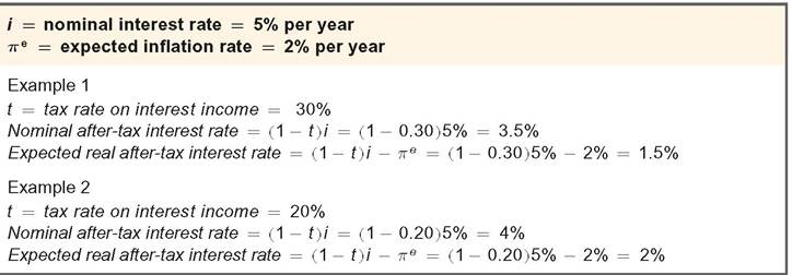
policy changes don't significantly affect the capital stock or employment. Later we relax the fixed-output assumption and discuss both the classical and Keynesian views about how fiscal policy changes can affect output.
In general, fiscal policy affects desired consumption, Cd, primarily by affecting households' current and expected future incomes. More specifically, fiscal changes that increase the tax burden on the private sector, either by raising current taxes or by leading people to expect that taxes will be higher in the future, will cause people to consume less.
For a given level of output, Y, government fiscal policies affect desired national saving, Sd, or Y — Cd — G, in two basic ways. First, as we just noted, fiscal policy can influence desired consumption: For any levels of output, Y, and government purchases, G, a fiscal policy change that reduces desired consumption, Cd, by one dollar will at the same time raise desired national saving, Sd, by one dollar. Second, for any levels of output and desired consumption, increases in government purchases directly lower desired national saving, as is apparent from the definition of desired national saving, Sd = Y — Cd — G.
To illustrate these general points, we consider how desired consumption and desired national saving would be affected by two specific fiscal policy changes: an increase in government purchases and a tax cut.
In Touch with Data and Research
Interest Rates
Although in our theoretical discussions we refer to "the" interest rate, as if there were only one, actually there are many different interest rates, each of which depends on the identity of the borrower and the terms of the loan. Shown here are some interest rates that appeared in Federal Reserve statistical release H.15 on February 23, 2021, and February 23, 2022.
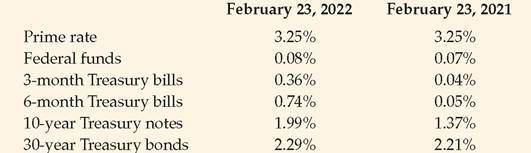
The prime rate is the basic rate that banks charge on loans to their best customers. The federal funds rate is the rate at which banks make overnight loans to one another. Treasury bills, notes, and bonds are debts of the U.S. government. With the exception of the prime rate, these interest rates vary continuously as financial market conditions change. The prime rate is an average of lending rates set by major banks and changes less frequently.
The interest rates charged on these different types of loans need not be the same. One reason for this variation is differences in the risk of nonrepayment, or default. Federal government debt is believed to be free from default risk, but there is always a chance that a business or bank may not be able to repay what it borrowed. Lenders charge risky borrowers extra interest to compensate
themselves for the risk of default. Thus the prime rate and the federal funds rate are higher than they would be if there were no default risk.
A second factor affecting interest rates is the length of time for which the funds are borrowed. The relationship between the life of a bond (its maturity) and the interest rate it pays is called the yield curve. The accompanying figure shows the yield curve in February 2022 and the yield curve one year earlier. Because longer maturity bonds typically pay higher interest rates than shorter maturity bonds, the yield curve generally slopes upward. We will discuss how interest rates relate to the maturity of a bond in the section "Time to Maturity" in Chapter 7.
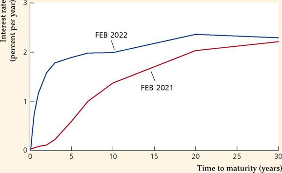
Although the levels of the various interest rates are quite different, interest rates go up and down together most of the time. As the graph shows, from February 2021 to February 2022, all of the interest rates rose, with the short-term rates rising generally more than the long-term rates. We will discuss a theory about that in Chapter 7, in Section 7.2, when we discuss the term structure of interest rates. As a general rule, interest rates tend to move together, so in our economic analyses we usually refer to "the" interest rate, as if there were only one.
Government Purchases. Suppose that current government purchases, G, increase by $10 billion, perhaps because the government increases military spending. Assume that this increase in G is temporary so that plans for future government purchases are unchanged. (Analytical Problem 5 at the end of this chapter looks at the case of a permanent increase in government purchases.) For any fixed level of output, Y, how will this change in fiscal policy affect desired consumption and desired national saving in the economy?
Let's start by finding the effect of the increased government purchases on consumption. As already mentioned, changes in government purchases affect consumption because they affect private-sector tax burdens. Suppose for example that the government pays for the extra $10 billion in military spending by raising current taxes by $10 billion. For a given total (before-tax) output, Y, this tax increase implies a $10 billion decline in consumers' current (after-tax) incomes. We know that consumers respond to a decline in their current incomes by reducing consumption, although by less than the decline in current income.[56] So, in response to the $10 billion tax increase, consumers might, for example, reduce their current consumption by $6 billion.
What happens to consumption if the government doesn't increase current taxes when it increases its purchases? The analysis in this case is more subtle. If the government doesn't increase current taxes, it will have to borrow the $10 billion to pay for the extra spending. The government will have to repay the $10 billion it borrows, plus interest, sometime in the future, implying that future taxes will have to rise. If taxpayers are clever enough to understand that increased government purchases today mean higher taxes in the future, households' expected future (after-tax) incomes will fall, and again they will reduce desired consumption. For the sake of illustration, we can imagine that they again reduce their current consumption by $6 billion, although the reduction in consumption might be less if some consumers don't understand that their future taxes are likely to rise.
What about the effects on desired national saving? The increase in government purchases affects desired national saving, Y — Cd — G, directly by increasing G and indirectly by reducing desired consumption, Cd. In our example, the increase in government purchases reduces desired consumption by $6 billion, which by itself would raise national saving by $6 billion. However, this effect is outweighed by the increase in G of $10 billion so that overall desired national saving, Y — Cd — G, falls by $4 billion, with output, Y, held constant.[57] More generally, because the decline in desired consumption can be expected to be less than the initial increase in government purchases, a temporary increase in government purchases will lower desired national saving.
To summarize, for a given current level of output, Y, we conclude that a temporary increase in government purchases reduces both desired consumption and desired national saving.
Taxes. Now suppose that government purchases, G, remain constant but that the government reduces current taxes, T, by $10 billion. To keep things as simple as possible, we suppose that each taxpayer receives the same amount (think of the country's 100 million taxpayers receiving $100 each). We call this a lump-sum tax cut. With government purchases, G, and output, Y, held constant, desired national saving, Y — Cd — G, will change only if desired consumption, Cd, changes. So the question is, How will desired consumption respond to such a lump-sum tax cut?
Again the key issue is, How does the tax cut affect people's current and expected future incomes? The $10 billion current tax cut directly increases current (after-tax) incomes by $10 billion, so the tax cut should increase desired consumption (by somewhat less than $10 billion). However, the $10 billion current tax cut also should lead people to expect lower after-tax incomes in the future. The reason is that, because the government hasn't changed its spending, to cut taxes by $10 billion today the government must also increase its current borrowing by $10 billion. Because the extra $10 billion of government debt will have to be repaid with interest in the future, future taxes will have to be higher, which in turn implies lower future disposable incomes for households. All else being equal, the decline in expected future incomes will cause people to consume less today, offsetting the positive effect of increased current income on desired consumption. Thus, in principle, a current tax cut—which raises current incomes but lowers expected future incomes—could either raise or lower current desired consumption.
Interestingly, some economists argue that the positive effect of increased current income and the negative effect of decreased future income on desired consumption should exactly cancel so that the overall effect of a current tax cut on consumption is zero! The idea that tax cuts do not affect desired consumption and (therefore) also do not affect desired national saving,[58] is called the Ricardian equivalence proposition.[59]
The Ricardian equivalence idea can be briefly explained as follows (see Chapter 15 for a more detailed discussion). In the long run, all government purchases must be paid for by taxes. Thus, if the government's current and planned purchases do not change, a cut in current taxes can affect the timing of tax collections but (advocates of Ricardian equivalence emphasize) not the ultimate tax burden borne by consumers. A current tax cut with no change in government purchases doesn't really make consumers any better off (any reduction in taxes today is balanced by tax increases in the future), so they have no reason to respond to the tax cut by changing their desired consumption.
| SUMMARY 5 | ||
| Determinants of Desired Nationc | ιl Saving | |
| An increase in | Causes desired national saving to | Reason |
| Current output, Y | Rise | Part of the extra income is saved to provide for future |
| Expected future | Fall | consumption. Anticipation of future income raises current desired |
| output | consumption, lowering current desired saving. | |
| Wealth | Fall | Some of the extra wealth is consumed, which reduces |
| Probably rise | saving for given income. An increased return makes saving more attractive, prob- | |
| interest rate, r | ably outweighing the fact that less must be saved to reach a | |
| Government | Fall | specific savings target. Higher government purchases directly lower desired |
| purchases, G | national saving. | |
| Taxes, T | Remain unchanged | Saving doesn’t change if consumers take into account |
| or rise | an offsetting future tax cut; saving rises if consumers | |
| don’t take into account a future tax cut and thus reduce current consumption. | ||
Although the logic of the Ricardian equivalence proposition is sound, many economists question whether it makes sense in practice. Most of these skeptics argue that, even though the proposition predicts that consumers will not increase consumption when taxes are cut, in reality lower current taxes likely will lead to increased desired consumption and thus reduced desired national saving. One reason that consumption may rise after a tax cut is that many—perhaps most—consumers do not understand that increased government borrowing today is likely to lead to higher taxes in the future. Thus consumers may simply respond to the current tax cut, as they would to any other increase in current income, by increasing their desired consumption.
The effects of a tax cut on consumption and saving may be summarized as follows: According to the Ricardian equivalence proposition, with no change in current or planned government purchases, a tax cut doesn't change desired consumption and desired national saving. However, the Ricardian equivalence proposition may not apply if consumers fail to take account of possible future tax increases in their planning; in that case, a tax cut will increase desired consumption and reduce desired national saving.
The factors that affect consumption and saving are listed in Summary table 5.
Application
In a world of globalized capital mobility, many governments in EMEs use tax incentives to signal openness to private investment and to respond to tax competition from other jurisdictions. Other EMEs use investment tax incentives to compensate for possible deficiencies in the investment climate and to counterbalance investment disincentives. Examples of the investment disadvantages that investors may face are poor infrastructure, obsolete laws, corruption, poor regulatory frameworks, bureaucratic complexities, and weak administrative systems.
We may be inclined to think that it is best to address the problem at its roots by reforming the legal framework, building administrative capacities, and enhancing the infrastructure. However, these solutions are quite costly and enduring, and tax incentives may provide short-term relief until the more fundamental structural remedies are carried out. Investors also need incentives to help compensate for inherent foreign exchange, political, credit, and legislative risk factors. Lastly, incentives could be carefully directed to sectors of economic activity that the government wishes to develop.
Against all of these benefits, tax incentives have costs and disadvantages that go beyond immediate loss of potential revenue. Advocates of the Ricardian equivalence proposition extend their argument from consumer to investor behavior, rendering them the strongest critics of investment tax incentives. They argue that in many instances investment spending would not increase much in response to a tax incentive, especially in EMEs where the poor investment environment, tax complexity, and the exposure to risk factors outweigh potential investment gains.[60] For example, it takes Nigerian companies approximately 908 hours each year to prepare, file, and pay their taxes, ranking Nigeria 179th in tax payment, according to the World Bank's Doing Business 2015 report. Further, the results of surveying 14,000 business executives in 148 economies by the World Economic Forum's 2014 Executive Opinion Survey reveal that financing and political stability are more important than tax considerations.
Moreover, preferential treatment of firms qualifying for tax incentives distorts efficient market equilibrium. As investors benefiting from incentives could possibly crowd out other investments, the aggregate investment capital stock may not increase, but simply move from one sector to the other. In addition to foregone revenue losses, the introduction of these tax incentives further complicates tax regulations, raising the administrative costs needed to collect taxes and to prevent fraudulent abuse of the incentive schemes.[61]
A study by the IMF[62] also reveals that tax incentives are not without social costs. They often lead to unfavorable cross-border tax competition, with the final result of providing private investors with windfall incomes at the expense of public expenditure and social benefits. Second, the desire to benefit from these preferential investment schemes can increase rent-seeking activities by individuals and businesses and may even increase corruption levels. The IMF study also notes
that since the capital stock may move toward larger or multinational firms, especially those operating within mobile sectors, the repercussions on employment and growth would be substantial for self-employed and small and medium enterprises, which have proved to be active engines of job creation.
In conclusion, investment tax incentives that are widely used by emerging market economies to attract private investment have had mixed effects. They only prove beneficial if the pertinent pre-conditions are met and the correct type of incentive is employed. In order to introduce rational tax policy tools, policymakers should first carefully weigh the costs and benefits of the incentives. For example, before introducing sector-specific incentives, revenue gains from additional employment taxes or taxes on inputs should be carefully weighed against the crowding out of other investments that may be more highly productive, job-generating, and taxable.
4.2