Growth and Financial Capital Flows
In a globalized economy, if the rates of return to capital differ across countries, we would expect capital to flow towards areas where its rate of return is higher. This simple observation has a number of important implications for growth theory.
First, it implies a very different pattern of economic growth in a financially integrated world. Our first task in this section isto illustrate the implications of international capital flows for economic growth and show how they significantly change transitional dynamics in the basic neoclassical growth model. Our second task is to highlight what new lessons can be derived from the analysis of economic growth in the presence of international capital flows. In particular, we will see that the presence of international capital flows raises a number of puzzles, most notably, the one emphasized by Lucas (1990): “Why Does Capital Not Flow from Rich to Poor Countries?”. We will see in the next section that this simple question helps us think about a range of important issues in economic growth and economic development. While a model of free flow of capital around the world is a good starting point, the existing evidence is not entirely consistent with such free flows. In particular, free flows of capital lead to a pattern of growth that appears counterfactual. Moreover, a large literature in international finance, starting with Feldstein and Horioka (1980), points out that there is much less net flows of capital from countries with high saving rates towards those with lower saving rates than a theory of frictionless international capital markets would suggest. In the next section we will briefly discuss why capital flows across countries may be hampered and what the implications of this are for cross-country growth dynamics.
19.1.1. A World Equilibrium with Free Financial Flows. Consider a world economy consisting of of J countries, indexed j = 1,...,J, each with access to an aggregate production function for producing a unique final good:

where Yj (t) is the output of this unique final good in country j at time t, and Kj (t) and Lj (t) are the capital stock and labor supply, Aj (t) is again the country-specific Harrod-neutral technology term.
As in the previous chapter, we assume that each country is “small” and ignores its effects on world aggregates. Throughout the section we assume that technological change occurs at a constant rate across countries, though there may be level differences in technology, that is,
where g is the common growth rate of technology in the world.
We assume that each country admits a representative household with the standard preferences at time t = O given by
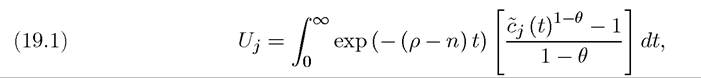
where Cj (t) is per capita consumption in country j at time t and we have imposed that all countries have the same time discount rate, ρ, and the same population growth rate n. Moreover, we assume that all countries start with the same population at time t = 0, which, 752
without loss of any generality, is normalized to 1, i.e., Lj (0) = 1 for all j = 1,...,J, so that  for all j. In addition, we assume that Assumption 4 from Chapter 8 is satisfied, i.e., ρ — n > (1 — θ) g.
The key feature of this economy is the presence of international borrowing and lending. Consistent with the permanent income hypothesis for individual consumption decisions, borrowing and lending will allow a smoother consumption profile for households (in particular for the representative household) in each country. But since the desire for a smoother consumption profile was one of the main reasons why the capital stock did not adjust immediately to its steady-state (or balanced growth path) value, the opportunities for international financial transactions will influence the dynamics of capital accumulation and growth.
More specifically, let Bj (t) ∈ R denote the net borrowing of country j from the world at time t. Let r (t) denote the world interest rate.
Free capital flows imply that this interest rate is independent of which country is borrowing and whether a country is borrowing or lending to others. Moreover, consistent with our assumption that each country is small relative to the world, all countries are price takers in the international financial markets, so they can borrow or lend as much as they like at this interest rate. Consequently, the flow resource constraint facing the representative household in each country will be somewhat different from that in subsection 18.2.2 and can be written as
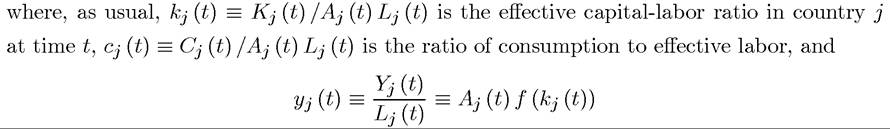
is income per capita, while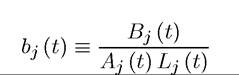
denotes the net borrowing normalized by effective labor. The most important feature of equation (19.2) is that, in contrast to all other resource equations we have encountered so far, it does not require domestic consumption and investment to be equal to domestic production. Instead, there are potential transfers of resources from the rest of the world, Bj (t), which can be used for consumption or investment. Conversely, the country may be transferring resources to the rest of the world, so that it consumes and invests less than its production. Naturally, once we allow for international borrowing and lending, we must ensure that each country, thus each representative household, satisfies an international budget constraint. For this purpose, let Aj (t) denote the international asset position of country j at time t. If Aj (t) 753
is positive, the country is a net lender and has positive claims on output produced in other countries, while if it is negative, the country is a net borrower. The flow international budget constraint for country j at time t can then be written as:

which simply states that the country earns the world interest rate, r (t), on its existing asset position A (t) (or accumulates further debt if the latter is negative) and in addition receives transfers B (t) from the rest of the world (or makes transfers to the rest of the world when B (t) is negative).
If transfers from the rest of the world exceed the interest earned on current assets, the asset position of the country deteriorates, that is, Aj (t) < 0. The no-Ponzi game condition we encountered in Chapter 8 now applies to the international asset position of acountry, and requires
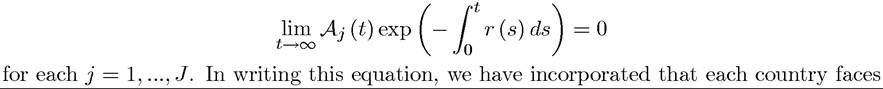
the world interest rate, r (t), at all points in time. The intuition for this expression is the same as the no-Ponzi game condition, (8.11) in Chapter 8.
As with the other variables, it is convenient to express the net asset position of the country in terms of effective labor units, so let us define
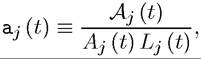
which implies that (19.3) can be rewritten as

and the no-Ponzi game condition becomes

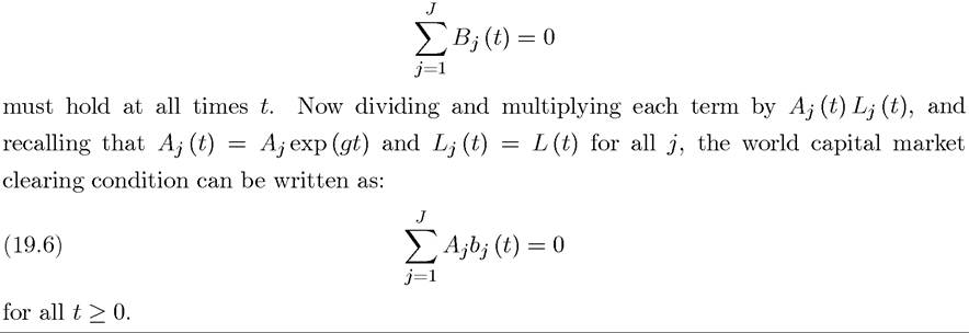
Naturally, the amount of borrowing and lending in the world has to balance out. This implies the world capital market clearing condition
With access to international capital markets, the problem of the representative household in each country can be written as maximizing (19.1) subject to (19.2), (19.4) and (19.5).
A world equilibrium is now defined as a sequence of normalized consumption levels, capital stocks and asset positions for each country, that is, and a time
path of world interest rates, such that each country’s allocation maximizes the
utility of the representative household in each country, and the world financial market clears,
that is, (19.6) is satisfied.
A steady-state world equilibrium is defined as a world equilibrium in which kj (t) and Cj (t) are constant and output in each country grows at a constant rate. As in previous chapters, we could alternatively refer to this allocation as a balanced growthpath rather than a steady-state equilibrium.
While the equilibrium of this world economy with free financial flows is quite straightforward to characterize, it is useful to present a number of simple intermediate results to emphasize a number of important economic ideas. The first one is the following proposition:
Proposition 19.1. In the world equilibrium of the economy with free flows of capital, we have that
where f0-1 (∙) is the inverse function of f' (∙) and r (t) is the world interest rate.
Proof. See Exercise 19.1.
?
This result is very intuitive. With free flows of capital, each firm in each country will stop renting capital only when its marginal product is equal to the opportunity cost, which is given by the world rental rate (the world interest rate plus the depreciation rate). Consequently, effective capital-labor ratios are equalized across countries. Note, however, that this does not imply equalization of capital-labor ratios. To the extent that two countries j and j0 have different levels of productivity, their capital-labor ratios are not,
and should not, be equalized. This is an important point to which we will return below.
The next proposition focuses on the steady-state world equilibrium.
PROPOSITION 19.2. Suppose that Assumption 4 is satisfied. Then in the world economy with free flows of capital, there exists a unique steady-state world equilibrium in which output, capital and consumption per capita in all countries grow at the rate g and effective capitallabor ratios are given by

Moreover, in the steady-state equilibrium, we have that
Proof.
See Exercise 19.2. ?At some level this result is very intuitive: with free capital flows, we have an integrated world economy. This integrated world economy has a unique steady-state equilibrium similar to that in the standard neoclassical growth model. This steady-state equilibrium not only determines the effective capital-labor ratio and its growth rate, but also the distribution of the available capital across different countries in the world economy. Even though this proposition is intuitive, its proof requires some care, to ensure that no country runs a Ponzi scheme and that this implies the normalized asset position of each country (and each household within each country), i.e., aj (t) for each j, must asymptote to a constant. This last feature is no longer the case when the model is extended so that countries differ according to their discount rates (see Exercise 19.2).
Let us next consider the transitional dynamics of the world economy. The analysis of transitional dynamics is simplified by the fact that the world behaves as an integrated economy rather than an independent collection of economies (see Exercise 19.2). Consequently, the following result is straightforward:
Proof. See Exercise 19.3.
?
Intuitively, the integrated world economy acts as if it has a single neoclassical aggregate production function, thus the characterization of the dynamic equilibrium path and of transitional dynamics from Chapter 8 applies. In addition, Proposition 19.1 implies that  is constant and the standard Euler equations imply tha
 is constant.
Therefore, both production and consumption in each economy grow in tandem.
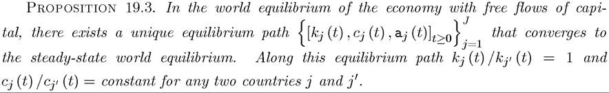
The following is an important corollary to Proposition 19.3:
COROLLARY 19.1. Consider the world economy with free flows of capital. Suppose that
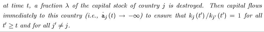
Proof. This is a direct implication of Propositions 19.1 and 19.3. The latter implies that there exists a unique globally stable equilibrium, while the former implies that at any point in the equilibrium we must have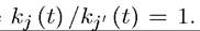 This is only possible by an immediate
inflow of capital into country j. ?
This result implies that in the world economy with free flows of capital, there are only transitional dynamics for the aggregate world economy, but no transitional dynamics separately for each country (in particular, kj (t) /kji (t) = 1 for all t and any j and j0). This is intuitive, since international capital flows will ensure that each country has the same effective capital-labor ratio, thus dynamics resulting from slow capital accumulation are removed. This corollary therefore implies that any theory emphasizing the role of transitional dynamics in explaining the evolution of cross-country income differences must implicitly limit the extent or the speed of international capital flows. The evidence on this point is mixed. While the amount of gross capital flows in the world economy is large, the Feldstein-Horioka puzzle still remains a puzzle—as we will see below, countries that save more also tend to invest more rather than lending this money internationally. One reason for this might be the potential risk of sovereign default by countries that borrow significant amounts from the world financial markets. Exercise 19.4 investigates this issue.
Although the implications of this corollary for cross-country patterns of divergence can be debated, its implications for cross-regional convergence are clear; cross-regional patterns of convergence cannot be related to slow capital accumulation as in the baseline neoclassical growth model. Exercise 19.5 asks you to apply this corollary to investigations of income convergence across U.S. regions and states.
19.2.