Households and Optimal Consumption and Money Demand
Assume that the economy consists of a continuum of identical households i, where i ∈ [0, 1]. Each household member is constrained to supply one unit of indivisible labor, and unemployment impacts all households in the same manner.8
The representative household chooses (aggregate) consumption and real money balances to maximize
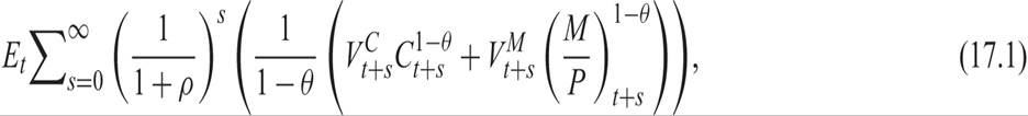
where ρ denotes the pure rate of time preference, θ is the inverse of the elasticity of intertemporal substitution, C is consumption, and M/P is real money balance.
In addition, VC and VM denote exogenous stochastic shocks in the utility from consumption and real money balances, respectively, and can be thought of as preference shocks.Consumption consists of differentiated goods and services indexed by a continuous index j, where j ∈ [0, 1]. The consumption bundle is thus given by
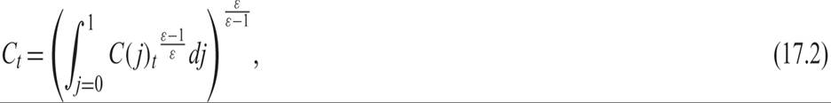
where ε is also a parameter of the preferences of the representative household, and more precicely, the elasticity of substitution between goods. We assume that ε > 1.
Expected utility is maximized subject to the sequence of expected budget constraints
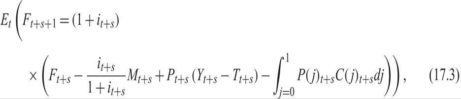
where Ft = Bt + Mt, denotes the financial assets held by the representative household, i is the nominal interest rate, B denotes one-period nominal bonds, M represents nominal money balances, Y is real noninterest income, T is real taxes net of transfers, and P( j) is the price of good j.
The household must also satisfy the transversality condition

The household must decide on the distribution of its consumption expenditure among the various goods and the intertemporal allocation of its total consumption expenditure and money demand.
The first problem requires the maximization of the consumption bundle (17.2) for any level of monetary expenditure. One can easily deduce that this implies
for any good j in the interval [0, 1], where P is the average price level, defined as
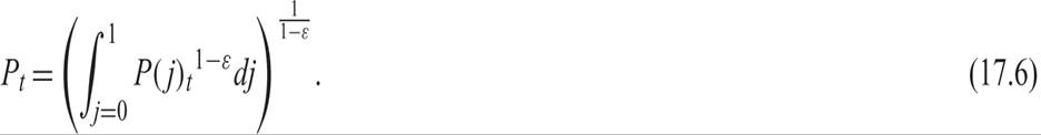
Equation (17.5) defines the demand for good j as a function of its relative price and the level of aggregate demand C.
In addition, when the household follows this optimal allocation policy, we also have that
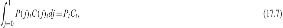
which suggests that total consumption expenditure can be written as the product of the aggregate consumption index and the aggregate price index. Substituting (17.7) in the sequence of expected budget constraints (17.3), we get

The solution to the intertemporal problem of the household can thus be derived from the first-order conditions for a maximum of (17.1), subject to (17.8). We then get
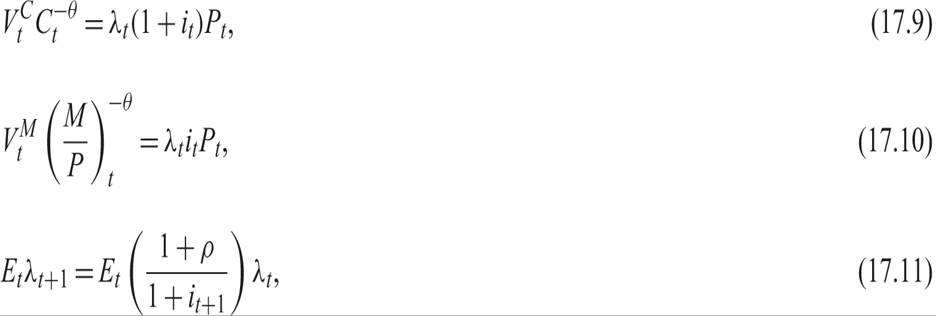
where λt is the Lagrange multiplier in period t. Equations (17.9)–(17.11) have the standard interpretations. Equation (17.9) suggests that at the optimum, the household equates the marginal utility of consumption to the value of savings. Equation (17.10) suggests that the household equates the marginal utility of real money balances to the opportunity cost of holding money. Equation (17.11) suggests that at the optimum, the real interest rate, adjusted for the expected increase in the marginal utility of consumption, is equal to the pure rate of time preference.
Eliminating λ from (17.9), (17.10), and (17.11) implies that
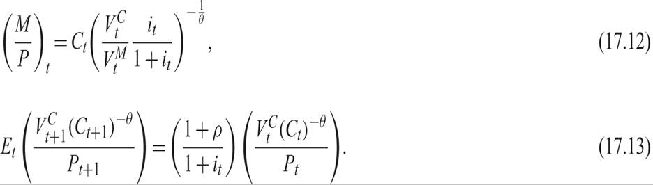
Equation (17.12) is the money demand function, which is proportional to consumption and a negative function of the nominal interest rate, and (17.13) is the familiar Euler equation for consumption.
Taking the logarithms of (17.12) and (17.13) yields
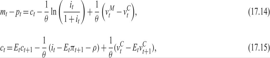
where lowercase letters denote natural logarithms, and πt = pt − pt−1 is the rate of inflation.9
We next turn to the behavior of firms in product markets.
17.3