Firms and Optimal Pricing and Production
Assume that output is produced by a set of firms denoted by a continuous index j defined in the interval [0,1]. Each firm produces a differentiated product under conditions of monopolistic competition.
All firms have access to the same production technology, denoted by the production function
where At > 0 and 0 < α < 1 are exogenous technological parameters, common to all firms; L( j)t is employment of labor by firm j in period t. The parameter α is constant, and At, exogenous productivity, is assumed to follow an exogenous stochastic process.
The optimal price of each firm, if it can choose its price in every period, is given by the maximization of its profits under the constraint of the production function (17.16) and the demand function for its product (17.5). Each firm takes the average price P, the nominal wage W( j), and the level of aggregate demand C as given.
The per period profits of firm j are given by

From the first-order conditions for a maximum of (17.17), under the constraints (17.16) and (17.5), the optimal price is determined as
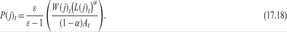
The optimal price is a fixed markup on the firm’s marginal cost, which equals the expression in the outer parentheses.
The marginal cost of production is the wage divided by the marginal product of labor. Because the marginal product of labor is decreasing with the level of employment, the marginal cost of production is an increasing function of employment and output.
The markup depends positively on the elasticity of substitution between goods in the preferences of consumers, which determines the price elasticity of demand of their product and therefore the profit margin of the firm.
In the case of perfect competition, the elasticity of substitution tends to infinity, and the price tends to marginal cost. In the case of monopolistic competition with ε > 1, as we have assumed, the optimal price is higher than the marginal cost of labor.10As all firms have the same production function and the same demand function for their product, they will all choose the same price if they face the same nominal wage W. Consequently, the price level will be defined as

If firms face different wages W( j), then they will choose different prices, and (17.19) denotes the average price as a function of the average of marginal unit labor costs. In either case, the price level is a fixed markup on marginal unit labor costs. It thus depends positively on nominal wages and employment, and negatively on exogenous productivity shocks.
Taking the logarithm of the production function (17.16) for the representative firm and equation (17.19) for the optimal price, we get
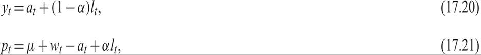
where at = ln At, and 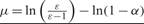 . Here a is the logarithm of the exogenous productivity shock, and the constant μ is the logarithm of the markup on marginal cost minus the logarithm of the coefficient of decreasing returns to the employment of labor.
From (17.21), we see that the higher the level of employment is, the higher will be the price level relative to nominal wages, as higher employment implies lower marginal productivity of labor. Because employment is positively related to output by the production function (17.20), higher output also implies higher prices relative to nominal wages. This can be seen by using (17.20) to substitute for employment in (17.21). One finds that

From (17.22), for given exogenous productivity at, firms will only produce more if prices rise relative to wages. The reason is that an increase in output results in higher unit labor costs, because of the diminishing marginal productivity of labor.
We next turn our attention to the labor market and the determination of nominal wages.
17.4