Wage Setting and Employment in a Model with Insiders and Outsiders

Nominal wages are set in a decentralized manner by insiders in each firm. Wages are set at the beginning of each period, before current productivity, current aggregate demand, and the current price level are known.

Thus, this model is characterized by nominal wage stickiness of the Gray [1976] and Fischer [1977b] variety. Prices are determined ex post by firms, given the contract wage, aggregate demand, the price level, and exogenous productivity a_t.

Following Blanchard and Summers [1986], assume that the number of insiders in each firm (who at the beginning of each period determine the contract wage) consists of an exogenous number of core insiders and those who were employed by the firm in the previous period. The objective of insiders is to set the maximum nominal wage, which—given their rational expectations about aggregate demand, the price level, and exogenous productivity—will minimize expected deviations of employment from the target level of the number of insiders. This target level is a weighted average of all those who were employed in period t − 1, and the exogenous set of core employees of each firm. Thus, this model is characterized by a state-dependent pool of insiders, as in Blanchard and Summers [1986]. The employment target of insiders in period t is determined by

alt=eq17-23.png>

where l( j)_t−1 is the logarithm of the number of those who were actually employed in the previous period; ( j) is the logarithm of the number of core employees of firm j, assumed exogenous; and δ is the weight of those recently employed relative to core employees, in the employment target of insiders.

The expectations on the basis of which wages are set depend on information available until the end of period t − 1, but not on information about aggregate demand, prices, and exogenous productivity in period t. On the basis of the above, let us assume that the objective of wage setters is to choose the path of maximum wages that would minimize deviations of the expected employment path from the expected path of the employment target of current insiders.

This can be modeled as a maximin problem. Insiders are assumed to choose the expected employment path that minimizes deviations from their target and to select the maximum wage path that satisfies their optimal employment path, subject to the optimal pricing decisions of firms. Thus, the first stage of the problem can be formalized as choosing the path of current and expected future wages that minimizes the following quadratic intertemporal loss function:

This is minimized subject to the sequence of optimal prices (17.21) and employment targets (j)_t, as defined in (17.23). Here, β = 1/(1 + ρ) < 1 is the discount factor, with ρ being the pure rate of time preference. As can be seen from (17.24), outsiders (i.e., the unemployed) have no influence on the wage-setting process.

We shall assume that the total number of core employees in the economy is always strictly smaller than the labor force. This assumption ensures that the natural rate of unemployment is strictly positive. We thus assume that

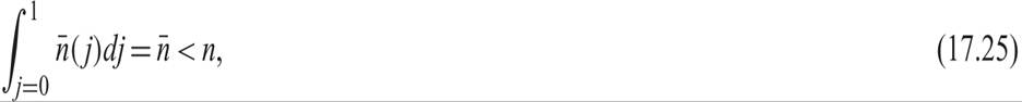
where n is the log of the labor force.

From the first-order conditions for a minimum of (17.24), wages are set at the maximum level that ensures that expected (log) employment by each firm satisfies

The implied contract wage can be derived by using the log-linear version of the optimal pricing condition (17.18) to substitute for employment in (17.26).

Integrating over j, expected aggregate employment must then satisfy

which is the same as (17.26) without the j index. Wage contracts that satisfy (17.27) encompass Gray-Fischer wage contracts and Blanchard-Summers wage contracts as special cases.

With the standard Gray-Fischer contracts, δ = 0, as past employment does not exert any separate influence on the wage-setting process. Only core employees would matter in Gray-Fischer contracts. Setting δ = 0 in (17.23), nominal wages in Gray-Fischer contracts would be set at the maximum level that ensures

With Blanchard-Summers contracts, there is no consideration of the effects of current contracts on expected employment beyond period t. This is equivalent to setting β = 0 in (17.27), that is, to assuming myopic behavior. Setting β = 0 in (17.27) implies that nominal wages would be set to ensure that

This equation is identical to equation (3.2) in Blanchard and Summers [1986]. Nominal wages with Blanchard-Summers contracts would be set at the maximum level that ensures that expected employment equals a weighted average of core employees and those recently employed, without consideration for the effects on future employment.

In our more general dynamic model, wages are set at the maximum level that ensures that expected employment in period t is given by (17.27), which also depends on expected employment in period t + 1. This is because expected employment at t will affect the number of insiders who will negotiate wages for period t + 1. Thus, in our model, current labor market insiders are forward looking, in that they set nominal wages to achieve an employment target that depends on core employees, those previously employed, but also on those expected to be employed in the future.

17.4.1 Wage Determination, Unemployment Persistence, and the Phillips Curve

To solve (17.27) for expected employment, define the forward expectations operator F as

We can then rewrite (17.27) as

Equation (17.29) can be rearranged as

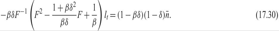
It is straightforward to show that if 0 < β < 1 and 0 < δ < 1, the characteristic equation of the quadratic in the forward shift operator (in large parentheses) has two distinct real roots, which lie on either side of unity. The two roots satisfy

Using (17.31), we can rewrite (17.30), as

Assuming λ₁ is the smaller root, we can solve (17.32):

Equation (17.33), which is the rational expectations solution of (17.27), determines the path of expected employment aimed at by the wage setting behavior of insiders.

It is straightforward to show that λ₁, the coefficient that determines the persistence of expected unemployment, is equal to δ, the relative weight of recent employees in the wage-setting process. From (17.31), which defines the two roots, it follows that because λ₂ = 1/βλ₁, it follows that

Thus, the degree of persistence of employment λ₁ is equal to the weight of recent employees relative to core employees in the wage-setting process δ, exactly as suggested by Blanchard and Summers [1986].

The expected employment equation (17.33) can be transformed into an expected unemployment equation in a straightforward manner. Subtracting (17.33) from the log of the labor force n, after some rearrangement, we get

where u_t ≃ n−l_t is the current unemployment rate, and is the natural rate of unemployment. The natural rate of unemployment in this model is defined in terms of the difference between the labor force and the number of core employees. This is the equilibrium rate toward which the economy would converge in the absence of shocks. Note that (17.35) also uses the fact that λ₁ = δ.

Actual employment is determined from the pricing and employment decisions of firms, after information about aggregate demand and productivity shocks has been revealed.

From the optimal pricing equation (17.21), to achieve the employment target (17.33), insiders will set the nominal wage to

Equation (17.36) uses the fact that λ₁ = δ. Substituting the wage-determination equation (17.36) in the optimal pricing equation of firms (17.21), the (log) price level will be determined by

Thus, prices will differ from the expectations of wage setters to the extent that there are unanticipated shocks to exogenous productivity and unanticipated shocks to aggregate demand. These shocks cause firms to determine employment at a different level than the one aimed at and expected by wage setters.

It is straightforward to transform (17.37) into an expectations-augmented Phillips curve.

where π_t = p_t −p_t−1 is the inflation rate, u_t ≃ n−l_t is the unemployment rate, n is the log of the labor force, and is the natural unemployment rate. Equation (17.38) is the expectations-augmented Phillips curve in this model. It is a dynamic version of a traditional expectations-augmented Phillips curve, in the sense that inflation depends on prior inflationary expectations but also on both current and past deviations of unemployment from its natural rate.

According to (17.38), current inflation differs from prior expectations of inflation to the extent that there are unanticipated shocks to exogenous productivity and unanticipated shocks to aggregate demand. These shocks cause the unemployment rate to differ from the target unemployment rate of wage setters. The dynamics arise because of the assumption that the target unemployment rate of wage setters is a weighted average of the past and the natural unemployment rate, due to the composition of labor market insiders. Note that when there is no persistence in the number of labor market insiders (i.e., when δ = 0), (17.38) takes the form of a standard expectations-augmented Phillips curve, like the one analyzed in chapter 15.

17.4.2 The Relation between Output and Unemployment Persistence

It is also clear from this model that only unanticipated shocks to exogenous productivity and aggregate demand cause unemployment to deviate from its expected path, as determined by the behavior of wage setters and summarized in (17.35). Note that if (17.35) holds, and wage setters have rational expectations, the unemployment rate follows

where is a white noise process, encompassing unanticipated productivity and demand shocks.

Hence, deviations of current unemployment from its natural rate will display persistence equal to δ, the weight of past employees on the wage-setting process. In fact, deviations of unemployment from its natural rate will follow an AR(1) process of the form

The persistence of employment and unemployment will also be translated into persistent output fluctuations.

Adding and subtracting (1 − α)(n − ) to the aggregate production function (17.20), we get

where

is the log of the natural rate of output. Equation (17.41) is an Okun [1962] type of relation, which suggests that fluctuations of output around its natural rate will be negatively related to fluctuations of the unemployment rate around its own natural rate. Because deviations of employment and unemployment from their natural rates display persistence, so will fluctuations in output. The propagation mechanism is the state dependence of the employment target of insiders in the labor market. Hence, deviations of output from its own natural rate will follow

Deviations of output from its natural rate will follow an AR(1) process as well, with the same degree of persistence δ as unemployment.

17.4.3 The Phillips Curve in Terms of Deviations of Output from Its Natural Rate

Substituting the Okun-type relation (17.41) in the expectations-augmented Phillips curve (17.38), we get an expectations-augmented Phillips curve defined in terms of deviations of output from its natural rate. This takes the form

To the extent that deviations of output from its natural rate are higher than what was anticipated at the time when wages were set, inflation is higher than anticipated, because employment and unit labor costs are higher than what was anticipated. Hence, firms increase prices by more than was previously expected.

Also note that when there is no persistence in the number of labor market insiders (i.e., when δ = 0), (17.44) takes the form of a standard expectations-augmented Phillips curve in terms of deviations of output from its natural rate.

17.5