The Implications of Staggered Pricing

Up to now we have assumed predetermined wage contracts and flexible prices. We can augment the model by introducing price stickiness as a additional nominal distortion. As in chapter 16, we shall concentrate on the Calvo [1983] model of staggered pricing.¹²

All firms are assumed to be able to automatically index their prices to the steady state inflation rate.

Under these assumptions, in period t, the expected future duration of any price contract is given by

From the definition of the price level in (17.6) and the fact that all firms that freely reset their prices in period t set the same price, it follows that

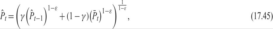
where is the price level relative to the steady state price level, and is the price set by the firms that freely reset their prices in the current period relative to the steady state price level.

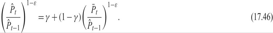
From (17.45), one can show that the dynamic adjustment of the price level relative to the steady state price level is determined by

In the steady state with inflation equal to π^*, we have that , and the price level evolves as

A log-linear approximation of (17.46) around the steady state price level yields

From (17.48), it follows that inflation exceeds its steady state rate if firms that set prices in the current period set them at a higher level than the average price of the previous period adjusted for steady state inflation.

17.5.1 Optimal Pricing with Staggered Price Adjustment

To analyze the adjustment of inflation, one has to examine how firms that can freely adjust prices in the current period decide on their optimal price, taking into account that for a period in the future, they may not be able to readjust their prices freely, while some of their competitors will have the option of readjusting their own prices at a rate different than core inflation.

The problem of the firm that decides on the price it is about to set in period t is to set the price that maximizes the expected present value of its profits, given that the probability of readjusting its price in any future period is equal to 1 − γ. Thus, all firms that readjust their prices in period t maximize

where 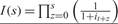, and Ŵ is the nominal wage divided by the steady state price level.

The maximization takes place under the constraints of their production function and the demand function for their product. These are given by

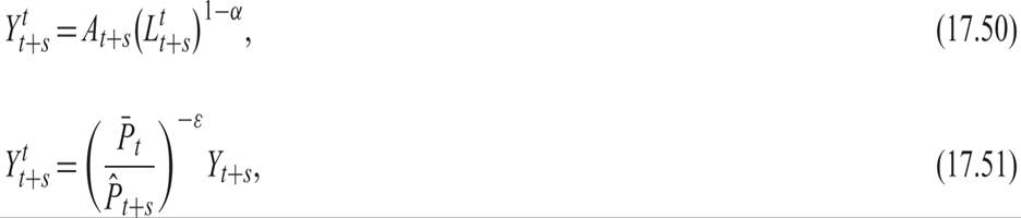
where and are respectively the volume of output and employment in period t + s of the firm that has set its prices freely in period t. The higher the relative price of the firm is in any period, the lower will be the demand for its product and thus the volume of its output and employment.

From the first-order conditions for a maximum, it follows that

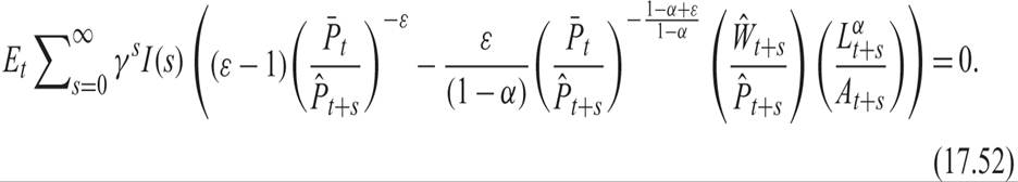
Equation (17.52) implies that the expected present value of revenues from the optimal price is equal to the expected present value of the marginal cost of production, augmented by the price markup ε/(ε − 1) of the firm.

Note that, as we have already seen in equation (17.19), if the firm could determine its prices in every period, the price of the product in each period would be equal to the marginal cost of production augmented by the same markup. However, if the firm cannot adjust prices freely in every period, as is assumed in the Calvo [1983] model, pricing follows the dynamic pricing rule (17.52).

Assuming that in the steady state, inflation is equal to π^* and all prices are equal to steady state prices, (17.52) can be transformed into logarithmic deviations from the steady state equilibrium, using a log-linear Taylor approximation. Thus, in logarithms, we have that

where , and . It follows that 0 < β, ω < 1.

Consequently, firms that freely reset their prices in period t will choose a price that corresponds to a weighted average of the current and expected future price levels, relative to the steady state price level, plus a margin μ on a weighted average of the current and expected future levels of real marginal costs. The discount factor of a future period t + s depends on the probability that the firm will not be able to reset its price in the future period t + s, which equals γ^s, times the discount rate β^s. Furthermore, the part of pricing that depends on the expected marginal cost of the firm depends negatively on the elasticity of demand for the product of the firm, through the parameter ω.

Using the future mathematical expectations operator F, (17.53) can be rewritten as

17.5.2 Inflation and Unit Labor Costs under Staggered Pricing

Substituting (17.54) in the equation for the adjustment of the average price level (17.48), we get

Multiplying both sides of (17.55) by 1 − βγF and rearranging, we get

Equation (17.56) is the equation of adjustment of the price level toward the steady state price level, which is a constant markup on the marginal cost of production.

From the price adjustment equation (17.56), we can deduce an equation for fluctuations in inflation. Expressing (17.56) as an inflation equation, we have

where π_t = p_t −p_t−1 is the rate of inflation. This equation implies that deviations of current inflation from steady state inflation are greater than discounted expected deviations of future inflation from steady state inflation, if the current marginal cost of labor plus the margin μ is higher than the current price level p. The reason is that firms able to set prices freely in the current period post larger price increases than the (discounted) expected future inflation, to offset the higher current marginal cost of labor.

Note that if all firms can adjust their prices freely and γ = 0, then the price level is always equal to the marginal cost of production augmented by the fixed markup μ, and inflation is equal to steady state inflation in all periods. Hence, the existence of a positive relation between inflation and employment in (17.57) requires staggered pricing in the form of a positive γ.

17.6