An Imperfectly Competitive Model of Aggregate Fluctuations

In this section, we examine in detail the structure of an imperfectly competitive model of aggregate fluctuations. The basic model that we analyze has much in common with the new classical model of chapter 14.

First, instead of perfectly competitive markets for goods and services, we assume that markets are characterized by conditions of imperfect (monopolistic) competition. Firms do not take prices as given; instead, they have the power to determine prices that maximize profits. Because of imperfect competition, in equilibrium, employment, real output, consumption, and real wages are determined at a lower level than in the corresponding competitive model, even when there is complete flexibility in prices and wages. By itself, this feature does not result in material differences from the competitive classical model with respect to the nature of aggregate fluctuations. If this was the only difference, we could well talk about an imperfectly competitive new classical model.

Second, we assume staggered price adjustment: Firms do not have the ability to change their prices at all times. This assumption is what leads to a model in which the price level adjusts gradually toward the equilibrium price level. As a result of gradual price adjustment, real variables deviate from their natural rates, and monetary shocks can have real effects.

16.1.1 The Representative Household

The problem of the representative household under monopolistic competition has one difference from the corresponding problem under perfect competition. The difference is that because of monopolistic competition, the household consumes differentiated products.

The representative household maximizes

where C is consumption, L is labor supply, and ρ is the pure rate of time preference.

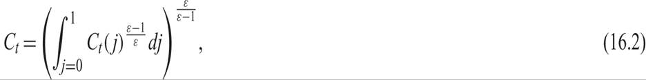
where ε is also a parameter of the preferences of the representative household; more precisely, it is the elasticity of substitution between goods. We assume that ε > 1.

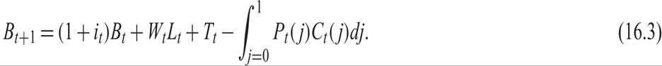
The sequence of budget constraints under which the household maximizes intertemporal utility is given by

The household must also satisfy the transversality condition:

where P(j) is the price of good j, W is the nominal wage, i is the nominal interest rate, B is a nominal one-period bond, and T is an exogenous transfer of nominal income to the household (dividends, government transfers, or taxes).

In addition to the decision about aggregate consumption and labor supply (which we have analyzed in section 14.1.1 of chapter 14), the household must now decide on the distribution of its consumption expenditure among the various goods. This requires the maximization of the consumption bundle (16.2) for any level of monetary expenditure. One can easily deduce that this implies

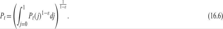
for any good j in the interval [0, 1], where P is the average price level, defined as

In addition, when the household follows this optimal allocation policy, we also have that

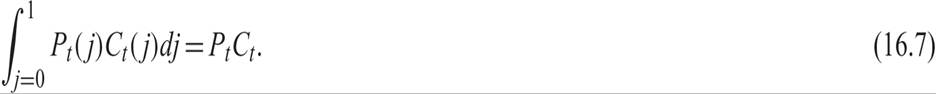
Equation (16.7) suggests that total consumption expenditure can be written as the product of the aggregate consumption index and the aggregate price index.

This sequence of budget constraints is the same as the sequence of budget constraints of the representative household in the competitive classical model of chapter 14. As a result, the first-order conditions for consumption and labor supply are analogous to the ones for the new classical model analyzed in chapter 14:

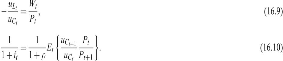
We assume, as in the new classical model without capital of chapter 14, that the per period utility function is additively separable and defined by

where 1/θ is the intertemporal elasticity of substitution in consumption, and 1/λ the Frisch elasticity of labor supply. Assuming that preferences take the form of (16.11), the first-order conditions (16.9) and (16.10) can be written in log-linear form as

where lowercase letters denote the logarithms of the corresponding variables, and π is the rate of inflation. Equations (16.12) and (16.13) are analogous to the ones in the new classical model in chapter 14.

16.1.2 The Representative Firm and Optimal Pricing

Assume that output is produced by a set of firms denoted by a continuous index j defined in the interval [0, 1]. Each firm produces a differentiated product under conditions of monopolistic competition. All firms have access to the same production technology, denoted by the production function

where A_t > 0 and 0 < α < 1 are exogenous technological parameters common to all firms, L( j) is employment of labor by firm j, the parameter α is constant, and A_t is assumed to follow an exogenous stochastic process.

The optimal price of each firm (if it can choose its price in every period) is given by the maximization of its profits under the constraint of the production function (16.14) and the demand function for its product (16.5). Each firm takes the average price P, the average wage W, and the level of total demand C as given.

The per period profits of firm j are given by

From the first-order conditions for a maximum of (16.15) under the constraints (16.14) and (16.5), the optimal price is determined as

The optimal price is a fixed markup on the firm’s marginal cost, which equals the expression in large parentheses. The markup depends on the elasticity of substitution between goods in the preferences of consumers, which determines the price elasticity of demand of their product and therefore the profit margin of the firm. In the case of perfect competition that we examined in chapter 14, the elasticity of substitution tends to infinity, and the price tends to marginal cost. In the case of monopolistic competition with ε > 1, as we have assumed, the optimal price is higher than the marginal cost of labor.¹

As all firms have the same production function and face the same nominal wage and the same demand function for their product, they will all choose the same price. Consequently, the price level is defined as

Taking the logarithm of the production function (16.14) for the representative firm and equation (16.16) for the optimal price, we get

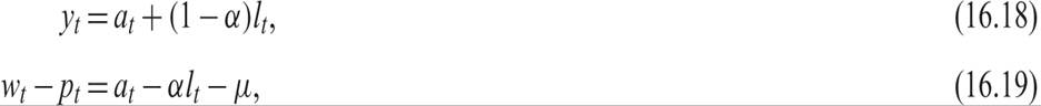
where 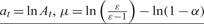, a is the logarithm of the exogenous productivity shock, and the constant μ is the logarithm of the markup on marginal cost minus the logarithm of the coefficient of decreasing returns to labor (which is equivalent to scale in this model).

16.1.3 Full Price Flexibility and the Natural Rate

Solving the model under the assumption of full flexibility of prices and wages, one can show that fluctuations in employment, output, consumption, and real wages are functions only of the exogenous shocks to productivity, while fluctuations in the real interest rate are a function of the expected change in productivity, just as in the new classical model under the assumption of perfect competition. Thus, under the assumption of full price flexibility, we can derive the natural rate solution of the model.

Because we have assumed that there is no investment or public consumption, equilibrium implies that labor supply would be equal to labor demand by firms, and consumption would be equal to output:

Equation (16.20) is the equilibrium condition in the labor market: The real wage makes labor supply by households equal to labor demand by firms. Equation (16.21) is the equilibrium condition in the output market: Output is equal to aggregate demand, which depends only on consumption.

The full model consists of equations (16.12), (16.13), (16.18), (16.19), and the equilibrium conditions (16.20) and (16.21). The model determines the natural rate solutions of employment, output, consumption, real wages, and the real interest rate as functions of the exogenous shock to productivity a.

The real interest rate is defined by the Fisher equation as

Solving the model for the five endogenous variables, we get

where , and ;

where , and ;

where , and ; and

Equations (16.23)–(16.26), along with the equilibrium conditions (16.20) and (16.21), determine the five endogenous real variables as functions of the exogenous productivity shock.

Output, consumption, and real wages are positive functions of the productivity shock a, and employment is a positive function of the productivity shock only if θ < 1 (i.e., only if the elasticity of intertemporal substitution is greater than one). If θ > 1, employment is a negative function of productivity, and if θ = 1, employment is independent of productivity. This applies because if θ < 1, the intertemporal substitution effect dominates the income effect, following a change in productivity and real wages. If θ > 1, the income effect dominates the intertemporal substitution effect, whereas in the case θ = 1, the two effects cancel each other out, and employment is not affected.

No other factor affects fluctuations in real variables. We see that, as in the competitive real business cycle (RBC) model of chapter 14, monetary factors (such as the money supply and nominal interest rates) have no effect on the evolution of real variables.

16.1.4 Inefficiency of the Natural Rate

However, this model has one significant difference from the competitive model of chapter 14. Because of monopolistic competition, which implies a positive margin of prices over marginal costs of firms, both employment and output (as well as consumption and real wages) are determined at a lower level than in the case of perfect competition. Monopolistic competition implies a distortion in the market of goods and services, which leads to lower equilibrium employment and output and to lower real wages than under perfect competition.²

If the productivity shock follows a stationary stochastic process with mean zero, then from (16.23), the log of the steady state employment level will be

If ε > 1, the steady state employment level will be lower than in the case of perfect competition.

Under perfect competition, goods are perfect substitutes in the preferences of consumers. Thus, steady state employment is

Because of imperfect competition, this model implies underemployment relative to a fully competitive model, even when there is full flexibility of prices and wages. Through (16.24) and (16.25), this underemployment implies that steady state output and steady state real wages will also be lower compared to perfect competition.

In all other respects, this model resembles the new classical competitive RBC model analyzed in chapter 14.

16.2