Staggered Price Adjustment and Aggregate Fluctuations

In contrast to the new classical models, in new Keynesian models, the assumption of fully flexible wages and prices is replaced by the assumption of gradual and only partial adjustment of nominal wages and prices toward their equilibrium values.

Various alternative new Keynesian models of gradual price adjustment under monopolistic competition have been developed in the literature. Let us concentrate on one of them, the Calvo [1983] model, which is based on staggered pricing.³

Following Calvo [1983], let us assume that firms cannot freely adjust their prices in every period at a rate different than steady state (or core) inflation. All firms are assumed to automatically adjust prices at the core inflation rate. However, for any firm, the probability of adjusting prices in any period at a rate different than core inflation is equal to 1 − γ, which is constant and independent of the length of time that has elapsed since the last such a price adjustment by the firm. Thus, in each period, a proportion 1 − γ of all firms adjust their prices freely at a rate different than core inflation, and the remaining proportion γ adjust their prices automatically at the rate of core inflation. This assumption has critical implications for the properties of the model, the nature of aggregate fluctuations, and the effects of monetary shocks and monetary policy.⁴

Under these assumptions, in period t, the expected future duration of any price contract is given by

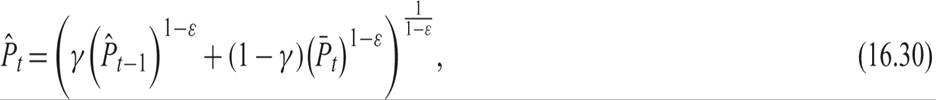
From the definition of the price level in (16.6) and the fact that all firms that reset their prices in period t set the same price, it follows that

where is the price level relative to the steady state price level, and is the price set by the firms that reset their prices in the current period relative to the steady state price level.

From (16.30), one can show that the dynamic adjustment of the price level relative to the steady state price level is determined by

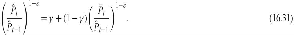
In the steady state with inflation equal to π^*, we have that , and the price level is given by

A log-linear approximation of (16.31) around the steady state price level yields

From (16.33), it follows that inflation exceeds its steady state rate if firms that set prices in the current period set them at a higher level than the average price of the previous period adjusted for steady state inflation.

16.2.1 Optimal Pricing with Staggered Price Adjustment

To analyze the adjustment of inflation, one has to examine how firms that can freely adjust prices in the current period decide on their optimal price. They must take into account that for a period in the future, they may not be able to readjust their prices freely, while some of their competitors have the option of readjusting their own prices at a rate different than core inflation.

The problem of the firm that decides on the price it is about to set in period t is to set the price that maximizes the expected present value of its profits, given that the probability of readjusting its price in any future period is equal to 1 − γ. Thus, all firms that readjust their prices in period t maximize

where and Ŵ is the nominal wage adjusted for the steady state price level.

The maximization takes place under the constraints of their production function and the demand function for their product. These are given by

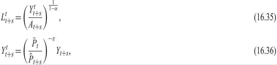
where and are the volume of output and employment, respectively, in period t + s for the firm that has set its prices in period t. The higher the relative price of the firm is in any period, the lower will be the demand for its product and thus the volume of its output and employment.

From the first-order conditions for a maximum, it follows that

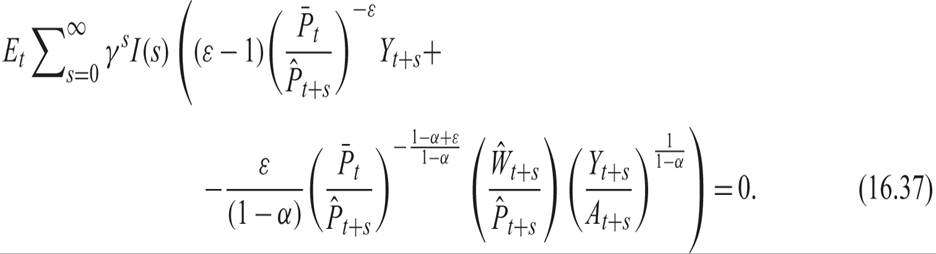
Equation (16.37) implies that the expected present value of revenues from the optimal price is equal to the expected present value of the marginal cost of production, augmented by the profit margin ε/(ε − 1) of the firm.

As we have already shown (equation (16.16)), if the firm could freely determine its prices in every period, the price of the product in each period would be equal to the marginal cost of production plus the same profit margin. However, if the firm cannot adjust prices freely in every period (as is assumed in the Calvo [1983] model), pricing follows the dynamic rule (16.37).

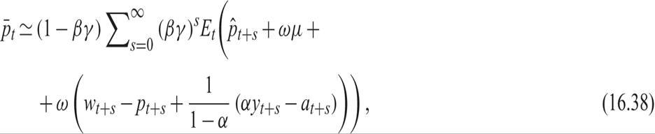
Assuming that in the steady state, inflation is equal to π^* and all prices are equal to steady state prices, (16.37) can be transformed to logarithmic deviations from the steady state equilibrium, using a log-linear Taylor approximation. Thus, in logarithms, we have that

where and .

Consequently, firms that freely reset their prices in period t will choose a price that corresponds to a weighted average of the current and expected future price levels (relative to the steady state price level) plus a margin μ on a weighted average of the current and expected future levels of real marginal costs. The discount factor of a future period t + s depends on the probability that the firm will not be able to reset its price in the future period t + s (which equals γ^s) times the discount rate β^s. Furthermore, the part of pricing that depends on the expected marginal cost of the firm depends negatively on the elasticity of demand for the product of the firm, through the parameter ω.

Using the future mathematical expectations operator F, (16.38) can be rewritten as

Substituting (16.39) in the equation for the adjustment of the average price level (16.34) we get that

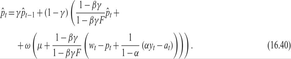
Multiplying both sides of (16.40) by 1 −βγF, after some rearrangements we get that

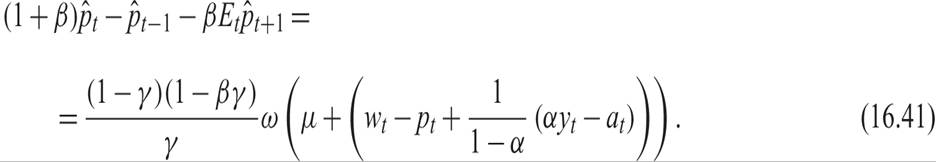
Equation (16.41) is the equation of adjustment of the price level toward the steady state price level, which is a constant markup on the marginal cost of production.

To examine the full model, we must introduce the equilibrium conditions in the markets for goods and services, labor, and money.

16.2.2 Equilibrium in the Market for Goods and Services and the New Keynesian IS Curve

Equilibrium in the market for good j implies that

As a result, equilibrium in the market for all goods requires that

where Y is aggregate output, defined in the same way as aggregate consumption C in equation (16.2).

Substituting the equilibrium condition (16.42) in the Euler equation for consumption (16.13), the logarithm of real output is determined by

Equation (16.43) is often referred to as the new Keynesian IS curve, as it is derived from the equilibrium condition for the market for goods and services. Recall that this is nothing more than the Euler equation for consumption, supplemented by the assumption that all output is consumed, and the same relation was derived in the new classical model of chapter 14. However, in contrast to the new classical model, where output is determined by aggregate supply, in this model, because of staggered pricing, output is determined by aggregate demand. Thus, it is the IS curve that drives output fluctuations.⁵

Compared to the conventional IS curve, (16.43) contains the rational expectation about future real output and explicitly depends on the real and not the nominal interest rate. Its theoretical advantage over the conventional IS curve is that it has been derived from explicit microeconomic foundations. Thus, its parameters depend on deep structural parameters, such as the pure rate of time preference of the representative household ρ and the intertemporal elasticity of substitution of consumption 1/θ, which are assumed to be invariant to policy. Hence, the new Keynesian IS curve is not subject to the Lucas [1976] critique, unlike the traditional IS curve.

16.2.3 Labor Market Equilibrium and the New Keynesian Phillips Curve

We next turn to the equilibrium condition in the labor market. Assume that, in contrast to product prices, which adjust gradually, nominal wages adjust immediately to equate the demand and supply of labor in each period. This assumption is made for reasons of analytical simplicity. Thus, the only nominal stickiness analyzed in this version of the new Keynesian model is the gradual adjustment of prices rather than wages.

Due to the gradual adjustment of prices, firms produce so as to satisfy aggregate demand at the given prices in each period. Aggregate output is determined by aggregate demand and differs from its natural rate, which is the level that would prevail if there was immediate price adjustment by all firms.

As a result, aggregate output, employment, consumption, real wages, and the real interest rate differ from their natural rates and display fluctuations that, as we shall show, depend on nominal as well as real disturbances.

From the price adjustment equation (16.41), we can deduce an equation for fluctuations in inflation. Expressing (16.41) as an inflation equation, we have that

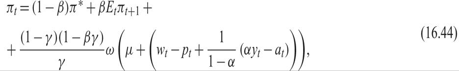
where π_t = p_t −p_t−1 is the rate of inflation. Equation (16.44) implies that deviations of current inflation from steady state inflation are greater than discounted expected deviations of future inflation from steady state inflation, if the current marginal cost of labor plus the margin μ is higher than the current price level p. The reason is that firms able to set prices in the current period post larger price increases than (discounted) expected future inflation, to offset the higher current marginal cost of labor.

The assumption of equilibrium in the labor market means that we can substitute the real wage in (16.44) from the first-order condition (16.12) for the representative household. Using (16.12), the condition for equilibrium in the market for goods and services (c = y), and the production function (16.18), (16.44) can be rewritten as

where y^N is the natural rate of real output (i.e., the output that would be produced if there was full flexibility of prices); y^N is given by (16.24). The parameter κ is defined by

Equation (16.45) is referred to as the new Keynesian Phillips curve and constitutes the second key behavioral equation of this imperfectly competitive new Keynesian DSGE model.

Deviations of output from its natural rate cause inflation to rise relative to expected future inflation because higher output implies a higher current real marginal cost of labor. This induces firms that have the opportunity to change their current price to post price increases that exceed discounted expected future inflation.

Like the new Keynesian IS curve, the new Keynesian Phillips curve has been derived from explicit microeconomic foundations, and its parameters are functions of the deep structural parameters describing the preferences of households, the technology of production, and the price-setting technology. One can confirm this by looking at the parameters that determines κ in (16.46).

Thus, the new Keynesian Phillips curve is also relatively impervious to the Lucas [1976] critique, although one could argue that the parameter γ of the price-setting technology may not be invariant to radical shifts in monetary policy.

16.2.4 The Imperfectly Competitive Model with Staggered Pricing and the Taylor Rule

Equations (16.43) and (16.46), along with equations (16.24) and (16.26) for the natural rate of real output and the real interest rate, constitute the basic structure of the imperfectly competitive new Keynesian model.

Deviations of current inflation from discounted expected future inflation are determined by the new Keynesian Phillips curve (16.45) as a function of deviations of real aggregate demand and output from the natural rate of output.

Deviations of real output from its natural rate are determined by the new Keynesian IS curve, which depends on deviations of the real interest rate from its own natural rate. The new Keynesian IS curve can be expressed as

where the natural levels of output y^N and the real interest rate r^N are determined by (16.24) and (16.26), respectively.

To close the model, we must consider the determination of the nominal interest rate. In contrast to the full information new classical model, due to staggered price adjustment, fluctuations in real variables cannot be determined without reference to monetary factors. Monetary factors and monetary policy determine not only the price level and inflation, as in the new classical model, but also fluctuations in real variables, such as real output, consumption, employment, real wages, and the real interest rate.

We shall analyze the model under the assumption that the central bank follows a Taylor [1993] rule of the form

where ϕ_π and ϕ_y are positive coefficients, and v is an exogenous stochastic disturbance in the nominal interest rate rule. Note that the constant in this rule is equal to ρ + π^*, the target steady state nominal interest rate consistent with steady state inflation equal to π^*.⁷

This monetary policy rule, which plays the role of the LM curve in traditional Keynesian models, implies a countercyclical monetary policy. When inflation is above π^*, the central bank increases nominal interest rates to reduce aggregate demand and nudge inflation toward π^*. When employment is low (i.e., when output is lower than its natural rate), the central bank reduces nominal interest rates to increase aggregate demand and nudge output and employment toward their natural rates.

As in the case of the Wicksell rule analyzed in chapter 14, this feedback interest rate rule does not result in inflation and price level indeterminacy if the Taylor principle is satisfied (i.e., if the reaction of nominal interest rates to inflation is sufficiently pronounced).⁸

Equations (16.45), (16.47), and (16.48) constitute the three key equations of the new Keynesian model with staggered pricing. These three equations—the new Keynesian Phillips curve, the new Keynesian IS curve, and the Taylor rule for nominal interest rates—determine deviations of output from its natural rate, deviations of inflation from the target of the central bank π^*, and the nominal interest rate i. All other nominal and real variables in the model are functions of these three variables.

16.2.5 Real and Monetary Shocks and Aggregate Fluctuations

Having now fully described the new Keynesian model with staggered pricing, we can analyze how nominal and real disturbances induce aggregate fluctuations.

The stochastic disturbance in the nominal interest rate is assumed to follow a stationary AR(1) process of the form

where 0 < η_v < 1, and is a white noise process.

The productivity shock a is also assumed to follow a stationary AR(1) process of the form

where 0 < η_a < 1, and is a white noise process.⁹

The full model consists of the new Keynesian Phillips and IS curves (16.45) and (16.47), the Taylor rule (16.48), the exogenous stochastic processes (16.49) and (16.50), and the equation for the determination of the natural real interest rate (16.26). Thus, the model can be written as

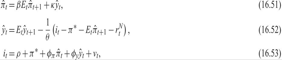
where = π − π* and denote the deviations between current and target inflation and between the current (log) real output and its natural rate.

The percentage deviation between current real output and its natural rate is often referred to as excess output, and its opposite is referred to as the output gap. When excess output is positive, the economy produces more than its natural rate; when it is negative (i.e., the output gap is positive), it produces less than its natural rate.

The natural real rate of interest r^N is determined by (16.26) and depends only on the expected change in the productivity shock and the pure rate of time preference.

The dimensions of the model can be reduced by substituting the Taylor rule for the nominal interest rate in the new Keynesian IS curve (16.52) and solving for excess output. This substitution results in an aggregate demand function of the form

Combined with the new Keynesian Phillips curve (16.51), (16.54) can help determine excess output and inflation as functions of the productivity shocks affecting the natural real rate of interest and the monetary shocks affecting the nominal interest rate rule.

One way to solve the dynamic system of (16.51) and (16.54) is the method of substitution, which requires substituting out for one of the endogenous variables, solving for the other, and then determining the variable that was originally substituted out. Another method is to express the two equations as a system, and use a systems method like the Blanchard and Kahn [1980] method. Both methods yield the same results; thus, we shall confine ourselves to the more intuitive substitution method.¹⁰

The substitution method involves substituting out for excess output from (16.54) into (16.51). After some rearrangement, this will result in an inflation equation of the form

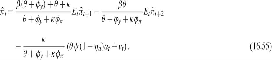
As can be seen from (16.55), deviations of inflation from steady state inflation depend on expectations about future inflation deviations, productivity shocks (which affect the natural real rate of interest), and nominal interest rate shocks. Recalling the definition of κ in (16.46), one can see that the parameters determining the inflation process depend on the preferences of the representative household θ, λ, ε, and ρ; the technology of production α; market structure ε; the price adjustment mechanism γ; and the parameters of the Taylor rule ϕ_π and ϕ_y.

Because inflation is a non-predetermined variable, both roots of (16.55) must be less than unity (inside the unit circle), which requires that the sum of the coefficients of the future expectations of inflation in (16.55) is less than one. Thus, for a stable inflation process, a necessary and sufficient condition is

Under the assumption that the coefficients of the Taylor rule ϕ_π and ϕ_y are positive, after some rearrangement of (16.56), one can see that a necessary and sufficient condition for a stable inflation process is

Hence, for a stable inflation process, the Taylor principle, as implied by (16.57) must hold. The reaction of nominal interest rates to current inflation must be sufficiently high to satisfy (16.57). For example, if the reaction of the nominal interest rate to excess output is zero (ϕ_y = 0), then the reaction of nominal interest rates to inflation must exceed unity.

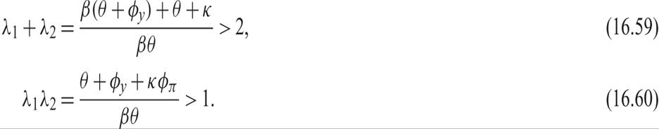
Assuming that the central bank policy satisfies (16.57), (16.55) can be solved forward for inflation, which is a non-predetermined variable. Inflation will be determined by

where 1/λ₁ and 1/λ₂ are the two roots of the inflationary process (16.55), which are both less than one if the Taylor principle (16.51) is satisfied. The inverses of these roots, λ₁ and λ₂, are both greater than one and are defined by

Inflation depends on future expectations of deviations of the natural real rate of interest from ρ and future expectations about nominal interest rate shocks v.

The closed-form solution for inflation, assuming that the two shocks follow AR(1) processes as in (16.49) and (16.50), takes the form

where

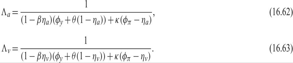
Note that the coefficients Λ_a and Λ_v depend negatively on the Taylor rule parameters ϕ_π and ϕ_y, which are in the denominator of both fractions. The larger the Taylor rule parameters are, the lower will be the impact of real and nominal shocks on deviations of inflation from the central bank target.

By substituting the solution for inflation in the new Keynesian Phillips curve (16.51), one can get the corresponding solution for the evolution of excess output. Excess output will be determined by

From (16.63), because the coefficients Λ_a and Λ_v depend negatively on the Taylor rule parameters ϕ_π and ϕ_y, the larger the Taylor rule parameters are, the lower will be the impact of real and nominal shocks on deviations of output from its natural rate.

Both monetary and real shocks affect fluctuations of real output and inflation in this model. Thus, the classical dichotomy does not hold. Persistent shocks to either nominal interest rates or productivity result in persistent deviations of inflation from the target of the central bank and persistent deviations of output from its natural rate. This new Keynesian model, unlike full information new classical models, can explain aggregate fluctuations caused by monetary shocks. These shocks are transmitted to real variables and persist over time through staggered pricing. Such monetary cycles cannot result from models with immediate and full adjustment of wages and prices, unless there is imperfect current information, as in models in the spirit of Lucas [1972].

16.2.6 The Divine Coincidence and Optimal Monetary Policy in the New Keynesian Model with Staggered Pricing

How different is the new Keynesian model with staggered pricing from the new classical models examined in chapter 14? Clearly, there are some key differences. For example, the natural rate of output and employment is suboptimally low because of imperfect competition; and there is staggered price adjustment, which results in short-run deviations of output, employment, and other real variables from their natural rates.

However, there are some important similarities as well. In the version of the model that we have examined, because nominal wages have been assumed fully flexible, employment fluctuations are only due to intertemporal substitution in labor supply, as in the new classical model. Thus, this version of the new Keynesian model cannot explain involuntary unemployment but only fluctuations of employment, much like the new classical model.

A second important similarity relates to optimal monetary policy. As we have seen in chapter 14, in a new classical model, optimal monetary policy is the one that continuously achieves the inflation target of the central bank, π^*. The same is true of the new Keynesian model with staggered pricing.

To see this, let us consider the new Keynesian Phillips curve (16.51). If the central bank could eliminate deviations of inflation from its target inflation rate π^*, then deviations of output from its natural rate would also be eliminated. Tackling fluctuations in inflation in this model has the effect of eliminating fluctuations in real variables as well. There is no trade-off between the stabilization of inflation and the stabilization of real variables around their natural rates. Blanchard and Gali [2007] have termed this property of the model the “divine coincidence.” In fact, to tackle the divine coincidence, they proposed that the new Keynesian model with staggered pricing be augmented with some form of exogenous real wage rigidity, which would break the link between the stabilization of inflation and the stabilization of output and employment.¹¹

The divine coincidence has important implications for optimal monetary policy and the Taylor rule. In fact, the optimal interest rate rule is one in which ϕ_π, the response of the interest rate to deviations of inflation from target, tends to infinity. This can be confirmed by examining (16.61) and (16.64), which are the closed-form solutions for inflation and the output gap, respectively. By allowing ϕ_π to tend to infinity in the Taylor rule, neither real nor monetary shocks cause deviations of inflation from target, and therefore output from its natural rate. The coefficients Λ_a and Λ_v tend to zero, and both inflation and the output gap are fully stabilized. This is the same as the optimal monetary policy rule in the new classical models of chapter 14.

Exercise 16.1 Solve the model consisting of equations (16.45), (16.47), and (16.48) using the Blanchard-Kahn method, and compare the solution to the results obtained by the substitution method. Assume that the exogenous shocks follow AR(1) processes, as in (16.49) and (16.50).

16.2.7 A Dynamic Simulation of the Model

To visualize the dynamic properties of the model summarized in (16.51)–(16.53), it is worth simulating it for particular parameter values and presenting the relevant impulse response functions.

Figures 16.1 and 16.2 present the dynamic effects of both monetary and real shocks for commonly used values of the parameters. The parameter values for this simulation are: θ = 1, λ = 1, ρ = 0.01, α = 0.333, ε = 6, γ = 0.667, ϕ_π = 1.50, ϕ_u = 0.125, η_a = 0.75, and η_v = 0.50. All real variables are defined as percentage deviations from their natural rates, and inflation is defined as percentage deviation from the target inflation of the central bank π^*.

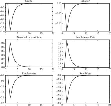
Figure 16.1 Impulse response functions of the staggered pricing model following a contractionary monetary shock.

Figure 16.2 Impulse response functions of the staggered pricing model following a positive productivity shock.

Figure 16.1 depicts the dynamic effects of a 1% positive shock ε^v in the nominal interest rate. This shock is a contractionary monetary shock, which leads to an increase of the nominal and the real interest rate and reduces excess output and inflation. This nominal shock does not affect the natural rate of real output, employment, real wages, or the real interest rate. However, actual real output, employment, and real wages decline relative to their natural rate, due to the reduction of aggregate demand and the staggered adjustment of prices. The economy gradually returns to its natural rate, as the effects of the monetary shock gradually die out.

Figure 16.2 depicts the dynamic effects of a 1% shock ε^a to productivity. This shock leads to a persistent rise in the natural rate of output, employment, and real wages, and a temporary fall in the natural real interest rate. However, due to the staggered adjustment of prices, actual real output, employment, and real wages do not rise as much as their natural rates. Hence, their deviations from their natural rates, depicted in figure 16.2, become negative. Inflation also falls below the target rate of the central bank. The negative discrepancy of output relative to its temporarily higher natural rate and the fall of inflation relative to the central bank target prompt a decline in nominal and real interest rates. Again, the economy gradually returns to its steady state equilibrium, as the effects of the real disturbance gradually die out.

Note the positive correlation between deviations of output from its natural rate and inflation from target, irrespective of the nature of the shocks hitting the economy. This is a result of the divine coincidence characterizing this model.

16.3