The Rotemberg Model of Convex Costs of Price Adjustment

An alternative to the Calvo [1983] model of staggered pricing is the Rotemberg [1982a,b] model of convex costs of price adjustment. For the representative monopolistically competitive firm, such as the one examined in section 16.1, the optimal price is given by

The optimal price is a constant markup on marginal costs.

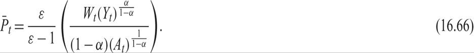
An increase in output increases the marginal costs of production for given wages because of the declining marginal productivity of labor. Hence, with higher output, the optimal price must rise.

In logs, (16.65) and (16.66) imply

where a_t = ln A_t, and 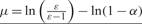. Here, a is the logarithm of the exogenous productivity shock, and the constant μ is the logarithm of the markup on marginal cost minus the logarithm of the coefficient implying decreasing returns to labor.

All firms are assumed to be facing convex costs of adjusting their posted prices. Rotemberg [1982a] assumes that firms balance the costs of deviating from their optimal price against the costs of changing their prices. In the model presented below, following Rotemberg, we assume that firms set current prices minimizing a quadratic cost function that penalizes both deviations of prices from the optimal price and the adjustment of prices over steady state inflation from period to period.

where p is the log of the actual price of the representative firm, and ξ is a parameter measuring the cost of price adjustment relative to the cost of deviations from the optimal price.

From the first-order conditions for the minimization of (16.68), it follows that

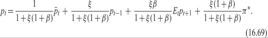
The current price, in logs, is a weighted average of the optimal price, the past price, and the expected future price. The firm is forward looking and anticipates the future costs of adjusting prices, so its current price depends not only on its past price but also on its expected future price. Because this is the representative firm, we can take p to be equal to the log of the price level.

Expressing (16.69) as an inflation equation, we get

where π_t = p_t − p_t−1 is the rate of inflation.

Inflation deviates from expected future inflation to the extent that the optimal price exceeds the current price. Substituting for the optimal price from (16.67), we get

where = π − π* is the deviation of inflation from steady state inflation.

From (16.71), deviations of current inflation differ from expected deviations of future inflation to the extent that the marginal cost of production plus the optimal price markup exceeds the current price. Using the labor and product market equilibrium conditions to substitute out for the real wage and employment, as well as the definition of the natural rate of output, we can express (16.71) as

where 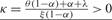and .

Hence, the analysis of the effects of monetary and real shocks in a new Keynesian model based on the Rotemberg model of costly price adjustment would be exactly the same as in the model based on Calvo-type staggered pricing.

16.4