Inequality, Credit Market Imperfections and Human Capital

The previous section illustrated how aggregate demand externalities can generate devel­opment traps. Investment by different firms may require coordination, leading to multiple equilibria.

Here I will illustrate these issues focusing on how the distribution of income and the organization of financial markets affect human capital investments. The models presented in this section will not only show the possibility of multiple steady states, but also shed light on more substantive questions related to the role of inequality and credit markets in the process of development. Although in this section I focus on human capital investments, the interaction between inequality and credit market problems influences not only human capital investments, but also occupational choices and other aspects of the organization of production. Nevertheless, the models focusing on the link between inequality and human capital are both more tractable and also constitute a natural continuation of the models of human capital investments we studied in Chapter 10.

21.6.1. A Simple Case With No Borrowing. When credit markets are imperfect, a major determinant of human capital investments will be the distribution of income (as well as the degree of imperfection in the credit markets). I start with a discussion of the simplest case in which there is no borrowing or lending, which introduces an extreme form of credit market problems. I will then enrich this model by introducing credit markets that allow borrowing and lending, but introduce credit market imperfections by making the cost of borrowing greater than the interest rate received by households engaged in saving.

The economy consists of continuum 1 of dynasties. Each individual lives for two periods, childhood and adulthood, and gets an offspring in his adulthood. There is consumption only 894

at the end of adulthood. Preferences are given by

where c is consumption at the end of the individual’s life, and e is the educational spending on the offspring of this individual. The budget constraint is

where w is the wage income of the individual. Notice that preferences here have the “warm glow” type altruism which we encountered in Chapter 9 and in Section 21.2 above. In particular, parents do not care about the utility of their offspring, but simply about what they bequeath to them, here education. As we have already seen, this significantly simplifies the analysis. Moreover, preferences are logarithmic, which as we have already seen, will imply a constant saving rate, here in terms of educational investments.

The labor market is competitive, and wage income of each individual is simply a linear function of his human capital:

Human capital of the offspring of individual i of generation t in turn is given by

where γ ∈ (0,1) and h ∈ (0,1) is some minimum level of human capital that the individual will attain even without any educational spending. Once spending exceeds a certain level (here set equal to 1), the individual starts benefiting from the additional spending and accumulates further human capital (though with diminishing returns since

This equation introduces a crucial feature necessary for models of credit market im­perfections to generate multiple equilibria or multiple steady states; a nonconvexity in the technology of human capital accumulation.

Given this description, the equilibrium is straightforward to characterize. Each individual will choose the spending on education that maximizes its own utility. This immediately implies the following “saving rate”:

This rule has one unappealing feature (not crucial for any of the results), which is that because parents derive utility from educational spending on their children, they will spend on education even when e⅛ (t) < 1, in which case educational spendings are in fact wasted (do not translate into higher human capital of the offspring).

To obtain stark results let us also assume that

895

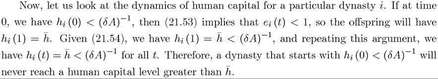
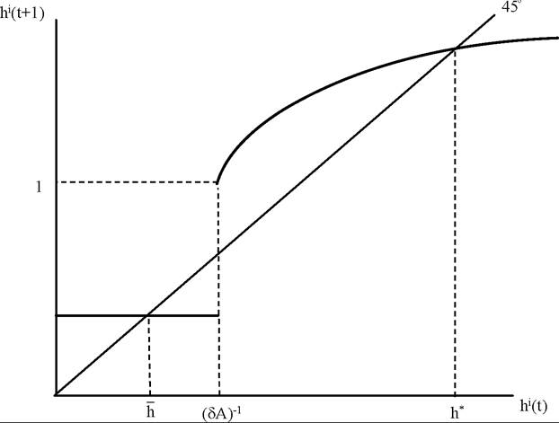
FIGURE 21.8. Dynamics of human capital with nonconvexities and no borrowing.

then the dynasty would have started with too much human capital and would decumulate human capital. Figure 21.8 illustrates the dynamics of individual human capital decisions. It of the dynamics in this model is so simple; the dynamics of the human capital of a single individual contains all the information relevant for the dynamics of the human capital and income of the entire economy. This is because there are no prices (such as the rate of return

896

to human capital or the interest rate) that are being determined in equilibrium here. For this reason, dynamics in this type of models are sometimes described as “Markovian”—because they are summarized by a Markov process without any general equilibrium interactions.

The most important implication of this analysis is that this simple model features poverty traps due to the nonconvexities created by the credit market problems. This is most clearly illustrated by contrasting two economies subject to the same technology and the same credit market problems, but starting out with different distributions of income. For example, imag­ine an economy with two groups starting at income levels hi and h∙₂ > h 1 such that (δA)^-1 < h2. Now if inequality (poverty) is high so that hi < (δA)^-i, a significant fraction of the population will never accumulate much human capital. In contrast, if inequality is lim­ited so that hi > (δA)^-i, all agents will accumulate human capital, eventually reaching h*. This example also illustrates that there are (many) multiple steady states in this economy. Depending on the fraction of dynasties that start with initial human capital (δA)^-i, any fraction of the population may end up at the low level of human capital,The greater is this fraction, the poorer will the economy be. At some level, there is a parallel between the multiplicity of steady states here and the multiple equilibria highlighted in the model of the previous section. Nevertheless, the differences are also noteworthy. In the model of the previous section, there are multiple equilibria in a static model. Thus nothing determines which equilibrium the economy will be in. At best, we can appeal to “expectations,” arguing that the better equilibrium will emerge when everybody expects the better equilibrium to emerge. One can informally appealed to the role of “history,” for example, suggesting that if an economy has been in the low investment equilibrium for a while, it is likely to stay there, but this argument is somewhat misleading.

the economy. But also, because multiple steady states are possible, the model can be useful for thinking about potential development traps.

Aside from providing us with a simple example of multiple steady states, this model shows the importance of the distribution of income in an economy with imperfect credit markets (here with no credit markets). In particular, the distribution of income affects which individuals will be unable to invest in human capital accumulation and thus influences the long-run income level of the economy. For this reason, models of this sort (including the one with imperfect capital markets we will study in the next section) are sometimes interpreted as implying that an unequal distribution of income will lead to lower output (and growth). In fact, the above example with two classes seems to support this conclusion. However, this is not a general result and it is important to emphasize that this class of models does not make specific predictions about relationship between inequality and growth.

21.6.2. Human Capital Investments with Imperfect Credit Markets. We now enrich the model of the previous subsection by introducing credit markets. The model I present here is a simplified version of the first Galor-Zeira model (Galor and Zeira, 1993). Each individual still lives for two periods. In his youth, he can either work or acquire education. The utility function of each individual is

where again c denotes consumption at the end of the life of the individual. The budget constraint is

where yi (t) is individual i’s income at time t. Note that preferences still take the “warm glow” form, but the utility of the parent now depends on monetary bequest to the offspring rather than the level of education expenditures. It will now be the individuals themselves 898

who will use the monetary bequests to invest in education. Also, the logarithmic formulation will once again ensure a constant saving rate equal to δ.

Education is a binary outcome, and educated (skilled) workers earn wage w_s while un­educated workers earn w_u. The required education expenditure to become skilled is h, and workers acquiring education do not earn the unskilled wage, w_u, during the first period of their lives. The fact that education is binary introduces the nonconvexity in human capital investment decisions. As demonstrated in Exercise 21.9, such nonconvexities are important for models with imperfect credit markets to generate multiple steady states.^[47]

Imperfect capital markets are modeled by assuming that there is some amount of mon­itoring required for loans to be paid back. The cost of monitoring creates a wedge between the borrowing and the lending rates. In particular, assume that there is a linear savings technology open to all agents, which fixes the lending rate at some constant r. However, the borrowing rate is i > r, because of costs of monitoring necessary to induce agents to pay back the loans (see Exercise 21.12 for a more micro-founded version of these borrowing costs).

Also assume that

which implies that investment in human capital is profitable when financed at the lending rate r.

Let us now consider an individual with wealth x. If x ≥ h, assumption (21.55) implies that individual will invest in education. If x < h, then whether it is profitable to invest in education will depend on the wealth of individual and the borrowing interest rate, i.

Let us now write the utility of this agent (with x x* converge to the greater wealth level Xs. As in the example without credit markets, there is a “poverty trap,” which attracts agents with low initial wealth. The distribution of income again has a potentially first-order effect on the income level of the economy. If the majority of the individuals start with x (t) < x*, the economy will have low productivity, low human capital and low wealth. Therefore, this model extends all of the insights of the simple model with no borrowing from the previous subsection to a richer environment in which individuals make forward-looking human capital investments. The key is again the interaction between credit market imperfections (which here make the interest rate for borrowing greater than the interest rate for saving) and inequality. As in the model of the previous subsection, it is straightforward to construct examples where an increase inequality can lead to either worse or better outcomes depending whether it pushes more individuals into the basin of attraction of the low steady state.

An important feature of the model of this subsection is that because it allows individuals to borrow and lend in financial markets, it enables us to investigate the implications of financial development for human capital investments. In an economy with better financial institutions, we may expect the wedge between the borrowing rate and the lending rate to be smaller, i.e., i to be smaller given r. With a smaller i, more agents will escape the poverty trap, and in fact the poverty trap may not exist (there may not be an intersection between

(21.56) and the 45 degree line where (21.56) is steeper). This shows that financial development not only improves risk sharing has demonstrated in Section 21.1, but in addition, by relaxing credit market constraints, it contributes to human capital accumulation.

Although the model in this section is considerably richer than that in the previous sub­section, a number of its shortcomings should also be noted. The most important shortcoming of the model is that, like the one in the previous subsection, it is essentially a partial equi­librium model. Multiple steady states are possible for different individuals as a function of their initial level of human capital (or wealth), but individual dynamics are not affected by general equilibrium prices. Models such as the second model presented in Galor and Zeira (1993), and those in Banerjee and Newman (1994), Aghion and Bolton (1997) and Piketty (1997) consider richer environments in which income dynamics of each dynasty (individual) is affected by general equilibrium prices (such as the interest rate or the wage rate), which are themselves a function of the income inequality at the time. Exercise 21.11 shows that the type of multiple steady states generated by the model presented here may not robust to the addition of noise in income dynamics—instead of multiple steady states, the long-run equilibrium then corresponds to a stationary distribution of human capital levels, though this stationary distribution will exhibit a large amount of persistence.^[48] In contrast, models in which prices determined in general equilibrium affect wealth (income) dynamics generate more robust multiplicity of steady states. The second potential shortcoming of the current model is that it focuses on human capital investments. Some development economists, such as Banerjee and Newman (1994), believe that the effect of income inequality on occupational choices is potentially more important than its effect on human capital investments. Exercise 21.13 presents a simplified version of the Banerjee-Newman model that emphasizes the role of occupational choice.

21.6.3. Heterogeneity, Stratification and the Dynamics of Inequality. The models in the previous two sections investigated the implications of credit market imperfec­tions and income distribution on human capital investments. In this subsection, I consider a slightly more general framework due to Benabou (1996a), which enables a study of the dy­namics of inequality and its costs for the efficiency of production resulting from its effect on human capital investments as a function of both the technology of production and how much stratification and segregation there is in the society. In particular, let me use a simplified version of Benabou’s (1996a) model where aggregate output in the economy at time t is given by

Y (t) = H (t),

where H (t) is an aggregate of the human capital of all the individuals in the society. In particular, normalizing the total population to 1 and denoting the distribution of human

capital at time t by μ_t (h), we have that

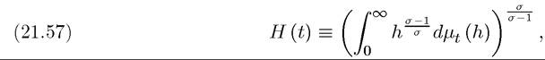
where the parameter σ measures the degree of complementarity or substitutability in the hu­

man capital of different individuals. When σ → ∞, the human capital of different individuals become perfect substitutes and H (t) is simply equal to the mean of the distribution of hu­man capital. For any value of σ ∈ (0, ∞), there is some amount of complementarity between the human capital levels of different individuals. For example, each individual performs a different task and overall output is a combination of these tasks. If some individuals have low human capital and are not very successful in the tasks they are supposed to perform, this reduces the productivity of other individuals in the society. The effect of heterogeneity of human capital on aggregate productivity, for a given mean level of human capital in the soci­ety, is most severe when the parameter σ is close to 0. Nevertheless, this formulation is also

general enough to allow for the case in which greater inequality is productivity-enhancing. In particular, even though this aggregator looks like the constant elasticity of substitution pro­duction function we have used many times in this book before, in contrast to that production function, it is defined for σ < 0 as well (whereas recall that the Dixit-Stiglitz aggregator is only defined for σ ≥ 0, see Exercise 21.14). When σ < 0, greater inequality for a given mean level of human capital increases the level of H (t) and thus productivity. For example, in the extreme case where σ → —∞, we obtain that H (t) = max⅛ {hi (t)}, that is, it is only the human capital of the highest human capital individual in the society that influences output. Since our interest here is on the potential costs of inequality on human capital investments, we will focus on the case where σ ≥ 0. In this case, a mean preserving spread of the human capital distribution μ will lead to a lower level of H (t) and a lower level of output.

The human capital of an individual from dynasty i at time t + 1 is given by

where B is a positive constant, hi (t) is the human capital of the individual’s parent, ξ_i (t) is a random shock affecting the individual’s human capital, and Ni (t) is the “average” human capital in the individual’s neighborhood. The human capital of the offspring is affected by his parent’s human capital either because of natural spillovers within the family or because the parent devotes some of his time to the rearing of his offspring and his time is more valu­able in child-rearing because of his higher human capital. In addition, the neighborhood and aggregate human capital levels, Ni (t) and H (t), affect the human capital of the individual through learning spillovers. For example, when the average human capital in the neighbor­hood is high, this may make it easier for the individual to acquire human capital. Aggregate human capital also enters this accumulation equation because the total (or average) level of human capital in the society may affect the type of knowledge that is available for the children to learn. The presence of this type of aggregate spillover means that a low level of H (t), for example because of high inequality, will not only reduce income today, but will also slow down further human capital accumulation.

Following Benabou (1996a), let us assume that the neighborhood human capital is also a constant elasticity of substitution aggregator, this time with an elasticity ε, i.e., 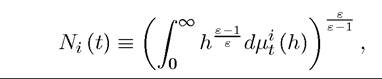where now μt (h) denotes the distribution of human capital in the neighborhood of individual i at time t. The presence of neighborhood human capital in the accumulation equation (21.58) implies that greater heterogeneity in the composition of a neighborhood might also have a negative effect on human capital accumulation. For example, presuming that ε ∈ (0, ∞), a mean preserving spread of neighborhood human capital will reduce the human capital of all 903

the offsprings. This structure of spillovers may be viewed as quite plausible, for example, because the presence of some low human capital children will slow down learning by those with higher potential (or because one “bad apple” will spoil the pack). This type of neighborhood spillovers may then suggest that segregation of high and low human capital parents in different neighborhoods might be beneficial for human capital accumulation. Whether or not this is so is one of the key questions that a model like this can answer.

The multiplicative structure in equation (21.58) gives a tractable evolution of the human capital distribution provided that the initial distribution of human capital is log normal and that the random shocks captured by ξ (t)s are log normal. In particular, let us assume the following log normal distributions for initial human capital and shocks

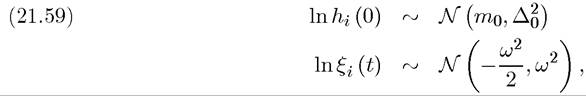
where N denotes the normal distribution, the draws of ξ_i (t) are independent across time and across individuals, and the distribution of ln ξ is assumed to have mean —ω²∕2 so that ξ has a mean equal to 1 (that is independent of its variance). It can then be established that the distribution of human capital within every generation will remain log normal, that is,

for some endogenous mean m_t and variance ∆_t, which will depend on parameters and the organization of society, for example, on the extent of segregation and integration (see Exercise 21.15). Consequently, the analysis of output and inequality dynamics in this economy boils down to characterizing the law of motion of m_t and ∆_t.

Let us now consider two alternative organizations. The first features full segregation so that each parent is in a neighborhood with identical parents. In that case, (21.58) becomes because the neighborhood human capital is the same as the parent’s human capital. The second features full mixing, so that each neighborhood is a mirror image of the entire society and thus for all neighborhoods we havewhere notice

that μ_t refers to the aggregate distribution. In this case, the accumulation equation becomes

The intuition above suggests that segregation might be preferable because it will prevent the adverse effects of neighborhood inequality on the human capital accumulation process. We will see, however, that this intuition is not entirely accurate, because whether there is segregation also affects the overall level of inequality in this society, and lack of segregation 904 may reduce long-run inequality leading to a better distribution of income and thus to better economic outcomes as a result.

With full segregation, it is straightforward to see that (see Exercise 21.16)

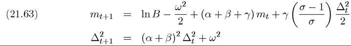
whereas with full integration, we have 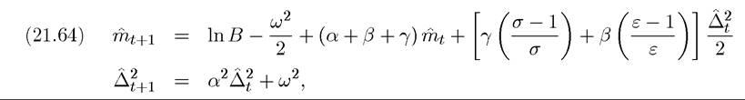where m_t andrefer to the values of the mean in the variance of the distribution under full integration.

A number of features about both of these equations are noteworthy. First, the expression for the mean of the distribution shows that there will be persistence in the distribution of human capital. This is because the human capital of the offsprings reflects the human capital of the parents (either through the direct affect on their own parent or through neighborhood and aggregate spillovers). This explains the autoregressive nature of the behavior of m_t. In addition, the dispersion of the parents’ human capital affects the mean of the distribution. In particular, when σ < 1 or when ε < 1, so that the degree of complementarity in the aggregate or the neighborhood spillovers is high, greater dispersion reduces the mean of the distribution of human capital. More interesting is the behavior of the variance of the distribution. When there is full segregation, the costs of heterogeneity in human capital accumulation resulting from neighborhood spillovers are avoided. But in return, the variance of log human capital is more persistent under segregation than full integration. In particular, it is straightforward to verify that when ε < 1, starting with the same m_t and ∆_t, we will have

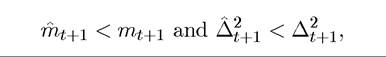
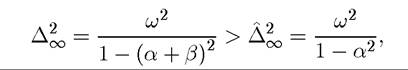
so that human capital in the next period is higher under segregation. But counteracting this, inequality is also higher and we know from the functional form in (21.57) that inequality has efficiency costs. So whether in the long run segregation or integration will generate greater output and a higher efficiency of production will depend on the dynamics of inequality and the exact structure of spillovers. To determine this, let us first find the long-run level of inequality under segregation and integration. Equations (21.63) and (21.64) immediately imply that these variances are given by

905

confirming that there will be greater inequality of human capital and income in this society with segregation of neighborhoods. The mean of the two distributions will also be different however. Let us suppose thatso that this steady state distribution exists

under both full segregation and full integration. Then we have

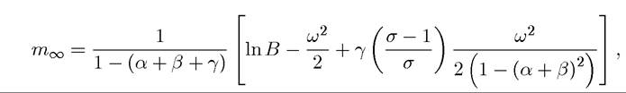
and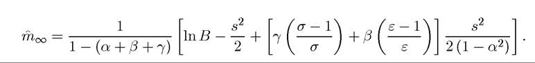

The comparison of these two expressions shows that the mean level of human capital in the long run may be higher or lower under full integration or full segregation. Using the production function above, taking logs on both sides of (21.57) and using log normality, we obtain that 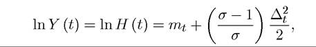so that long-run income levels under full segregation and full integration are

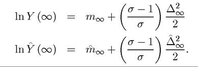
Consequently, depending on parameters long-run income levels may be higher or lower under full segregation and full integration (see Exercise 21.17).

This model therefore provides a richer framework for the analysis of the dynamics of income inequality than the models we have seen in the previous two subsections and also highlights various different costs arising from income inequality. Counterbalancing this rich structure is that the costs of inequality in this model are introduced in a reduced-form way. While the aggregator in (21.57) is plausible, one may wonder why there could not be segregation in production, so that high human capital individuals produce with other high human capital individuals, preventing the costs of inequality. One answer to this provided in Acemoglu (1997b), where individuals with different levels of human capital are matched with firms via a imperfect matching technology (see Exercise 21.18). Other, more technology­based justifications for (21.57) can also be provided. Another advantage of this framework is that its relative tractability makes it attractive for the study of political economy decisions, such as a voting over education budgets, and also for the analysis of issues such as education reform. These topics are addressed in Benabou (1996a,b).

21.7. Towards a Unified Theory of Development and Growth?

There has been a unified theme to the models discussed in this chapter (and even be­tween those discussed in this and the previous chapter). They have either emphasized the transformation of the economy and the society over the process of development or potential reasons for why such a transformation might be halted. This transformation takes the form of the structure of production changing, the process of industrialization getting underway, a greater fraction of the population migrating from rural areas to cities, financial markets be­coming more developed, mortality and fertility rates changing via health improvements and the demographic transition, and the extent of inefficiencies and market failures becoming less pronounced over time. In many instances this driving force is self-reinforced by the structural transformation that it causes. For example, in Section 21.1 and in the model of Section 17.6 in Chapter 17, economic development leads to financial deepening and this in turn enables a better allocation of resources and contributes to further growth and development. In all of the models, economic development is associated with capital deepening, that is, with greater use of capital instead of human labor (or combined with labor). Thus we can also approx­imate the growth process with an increase in the capital-labor ratio of the economy, k (t). This does not necessarily mean that capital accumulation is the engine of economic growth. In fact, previous chapters have emphasized how technological change is often at the root of the process of economic growth (and economic development) and thus capital deepening may be the result of technological change. Moreover, Section 21.4 emphasized how the crucial variable capturing the stage of development might be the distance of an economy’s technol­ogy to the world technology frontier. Since technological progress appears to play a crucial role in economic growth, we may also wish to take at least certain aspects of the technolog­ical changes taking place during the process of development as endogenous, especially when the link between development and changes in the extent of market failures is highlighted. Nevertheless, even in these cases, an increase in capital-labor ratio will take place along the equilibrium path and can thus be used as a proxy for the stage of development (though in this case one must be careful not to confuse increasing the capital-labor ratio with ensuring economic development). With this caveat in mind, in this section we take the capital-labor ratio as the proxy for the stage of development and for analytical convenience, we use the Solow model to represent the dynamics of the capital-labor ratio.

With the capital-labor ratio as the proxy for development, can we then construct a unified model where a single force drives the process of development and the structural transforma­tions spurred by this force contribute to the evolution of this driving force? Developing such a unified theory of development is certainly worthwhile. But I will not offer such a unified theory here. This is for two reasons. First, an attempt to pack many different aspects of

development into a single model will lead to a framework that is complicated and involved and I believe that relatively abstract representations of reality are more insightful. Second, the economic growth and development literatures have not made great progress towards such unified model. So while I believe there is room for thinking and constructing such unified theories of economic development, I do not think that one (or at least I) can do justice to this challenging task at this point in time and in this limited space.

Instead, I will provide a very reduced-form canonical model of development and structural change. This model is neither meant to be a unified theory of development and growth nor is it meant to be a model that will be informative about the details of the process of development. My purpose is different and more modest. I would like to bring out the common features of the models we have seen in this chapter, albeit in a very stylized and reduced-form manner.

Consider a continuous-time economy. Suppose that output per capita is given by

where k (t) is capital-labor ratio and x (t) is some “social variable,” such as financial devel­opment, urbanization, structure of production, the structure of the family etc. As usual, f is assumed to be twice continuously differentiable and also increasing in concave in k. Moreover, the social variable x potentially affects the efficiency of the production process and thus is part of the per capita production function in (21.65). As a convention we think of an increase in x as corresponding to structural change, such as a move from the countryside to cities, and thus suppose that f is not only increasing in k, but also in x. Naturally, not all structural change is beneficial, and certain aspects of the structural changes, such as pollution, may reduce productivity. But here for simplicity’s sake I focus on the case in which f is increasing in x, that is, the partial derivative f_x ≥ 0.

Let us assume a highly reduced-form model of social change represented by the differential equation

where g is also assumed to be twice continuously differentiable. Since x corresponds to structural change associated with development, g should be increasing in k, and in particular we assume that its partial derivative with respect to k is strictly positive, that is, g_k > 0. Moreover, standard mean reversion type reasoning suggests that g_x should be negative. If x is above its “natural level,” it should decline and if it is below its natural level, it should increase. Motivated by this, let us also assume that g_x < 0.

Capital accumulates according to the most basic Solow growth model is in Chapter 2, so that

908

where I have suppressed population growth and there is no technological change for simplicity. For a fixed x, capital naturally accumulates in an identical fashion to that in the basic Solow model. The structure of this economy is slightly more involved because x (t) also changes. Differential equations (21.66) and (21.67) provide a simple reduced-form representation of structural change driven by economic growth (capital accumulation).

To illustrate the types of dynamics and insights implied by this representation, first con­sider the case in which f_x (k, x) ? 0 so that the social variable x has no effect on productivity. Dynamics in this case are shown in Figure 21.10. The thick vertical line corresponds to the locus fori.e., it represents the zero of the differential equation (21.67). This

locus takes the form of a vertical line, since only a single value of, is consistent with steady state. The upward sloping line, on the other hand, corresponds to (21.66) and shows the locus of the values of k and x such thatIt is upward sloping, since g

is increasing in k and decreasing in x. The laws of motion represented by the arrows follow straightforwardly from (21.66) and (21.67). For example, when k (t) < ê*, (21.67) implies that k (t) will increase. Similarly, when x (t) is above the(21.66) implies

that x (t) will decrease. Given the laws of motion implied by the arrows, it is straightfor­ward to see that the dynamical system representing the equilibrium of this model is globally stable and starting with any k (0) > 0 and x (0) > 0, the economy will travel towards the unique steady state (k*,x*). Now consider the dynamics of a less-developed economy, that is, an economy that starts with a low level of capital-labor ratio, k (0), and a low level of the social variable, x (0). Then development in this economy will take place with gradual capital deepening and a corresponding increase in x (t) towards x*, which can be viewed as a reduced-form representation of development-induced structural change.

Next, consider the more interesting case in which f_x (k,x) > 0. In this case, the locus forwill also be upward sloping, since f_x > 0 and the right-hand side of

(21.67) is decreasing in k by the standard arguments (in particular, because of the fact that by the strict concavity of f (k, x) in k, f (k, x) /k > f (k, x) for all k and x, see Exercise 21.19) A steady state is again given by the intersection of the loci forand

Since both of these are now upward sloping, multiple steady states are possible as shown in Figure 21.11. These multiple steady states capture, in a very reduced- form way, the potential multiple equilibria arising from aggregate demand externalities or from the interaction between non-convexities and imperfect credit markets in Sections 21.5 and 21.6. The low steady state (k⁰,x⁰) corresponds to a situation in which the social variable x is low and thus productivity is low, and this makes the economy settle into an equilibrium with a low capital-labor ratio. In contrast in the high steady state (k*,x*), the high level of x supports greater productivity and thus a greater capital-labor ratio consistent with steady state. Moreover, it can be verified that both the low and the high steady states are typically

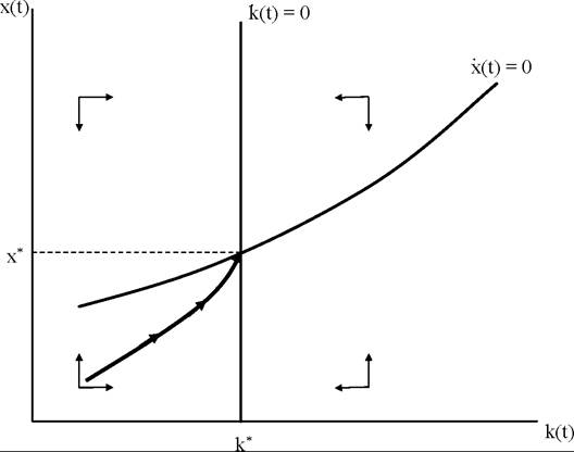
Figure 21.10. Capital accumulation and structural transformation without any effect of the “social variable” x on productivity.

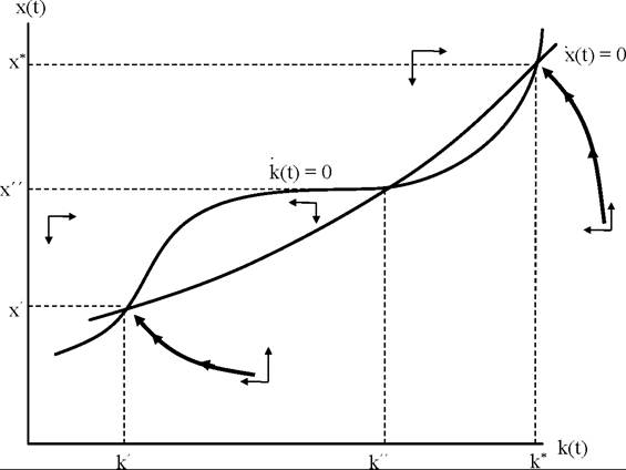
Figure 21.11. Capital accumulation and structural transformation with multiple steady states.

locally stable, so that starting from the neighborhood of one, the economy will converge to the nearest steady state and will tend to stay there. This highlights the importance of historical factors in the development process. If historical factors or endowments placed the economy in the neighborhood of the low steady state, the economy will converge to this steady state 910

corresponding to a “development trap”. Interestingly, this development trap is, at least in part, caused by lack of structural change (i.e., a low value of the social variable x).

Figure 21.11 makes it clear that such multiplicity requires the locus for k (t) /k (t) = 0 to be relatively flat, at least over some range. Inspection of equation (21.67) shows that this will be the case when f_x (k, x) is large, at least over some range. Intuitively, multiple steady-state equilibria can only arise when the social variable x has a large effect on productivity, so that the extent of structural change that the economy has already undergone should have a large effect on productivity.

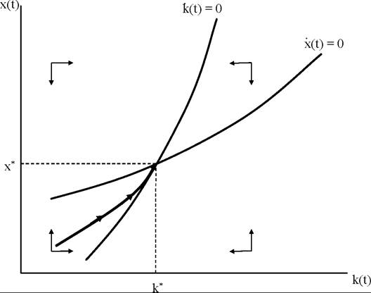
Figure 21.12. Capital accumulation and structural transformation when the “social variable” x affects but there exists a unique steady state.

More interesting than multiple steady states is the situation in which the same forces are present, but a unique steady state exists (like the models discussed in Section 21.6). The same reasoning suggests that this will be the case when f_x (k, x) is relatively small. 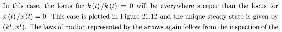differential equations (21.66) and (21.67). This figure shows that the unique steady state is globally stable (see Exercise 21.19 for a formal proof). Consider, once again, a less-developed economy starting with a low level of capital-labor ratio, k (0), and a low level of the social variable, x (0). The dynamics in this case are qualitatively similar to those in Figure 21.10. However, the economics is slightly different. Capital accumulation (capital deepening) leads to an increase in x (t) as before, but now this structural change also improves productivity as

in the models we have analyzed in Section 17.6 in Chapter 17 and in Sections 21.3 and 21.1 of this chapter. This increase in productivity leads to faster capital accumulation and there is a self-reinforcing (“cumulative”) process of development, with economic growth leading to structural changes facilitating further growth. However, since the effect of x on productivity is limited, this process ultimately takes us towards a unique steady state.

This reduced-form representation of structural change, therefore, captures some of the salient features we have emphasized in this chapter. It is not meant to be a unified model; on the contrary, rather than combining multiple dimensions of structural change, it presents an abstract representation emphasizing how the process of development, corresponding to capital accumulation, can go hand-in-hand with structural change, which may in turn increase productivity and facilitate further capital accumulation. The development of a truly unified model of economic development and the structural change associated with it is an area for future work.

21.8.