Multiple Equilibria From Aggregate Demand Externalities and the Big Push
I now present a simple model of multiple equilibria arising from aggregate demand externalities. The model is a version of Murphy, Shleifer and Vishny’s (1989) model of “big push”, which formalized ideas proposed by Rosenstein-Rodan (1943), Hirschman and Nurske, hat economic development can be viewed a move from one (Pareto inefficient) equilibrium to another, more efficient equilibrium.
Moreover, these early development economists argued that this type of move requires coordination among different individuals and firms in the economy, thus a big push. As already discussed in Chapter 4, multiple equilibria, literally interpreted, are unlikely to be the root cause of persistently low levels of development, since if there is indeed a Pareto improvement—a change that will make all individuals better off—it is unlikely that the necessary coordination cannot be achieved for decades or even centuries. Nevertheless, the forces leading to multiple equilibria highlight important economic mechanisms that can be associated with market failures slowing down, or even preventing, the process of development. Moreover, dynamic versions of models of multiple equilibria can 886lead to multiple state states, whereby once an economy ends up in a steady state with low economic activity, it may get stuck there (and there is no possibility of a coordination to jump to the other steady state). Models with multiple steady states will be discussed in the next section, where I will return to a further discussion of the difference between multiple equilibria and multiple steady states.
Murphy, Shleifer and Vishny consider the following two-period economy, t = 1 and 2. The economy admits a representative household with preferences given by
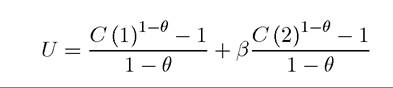
where C (1) and C (2) denote consumption at the two dates; β is the discount factor of the households; and θ plays a similar to before; 1∕θ is the intertemporal elasticity of substitution and determines how willing individuals are to substitute consumption between date 1 and date 2.
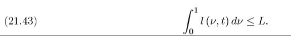
The representative household supplies labor inelastically and the total labor supply is denoted by L.The resource constraint for the economy is
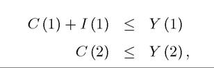
where I (1) denotes investment in the first date, Y (t) is total output at date t, and investment is only possible in the first date.
Households can borrow and lend, so their budget constraint can be represented as
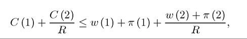
where π (t) denotes the profits accruing to the representative household, and w (t) is the wage rate at time t. R is the gross interest rate between periods 1 and 2. Although individuals can borrow and lend, in the aggregate the resource constraints have to hold, so R will be determined in equilibrium to ensure this.
As in the endogenous technological progress models in Part 4 and in the model of the previous section, the final good is assumed to be a constant elasticity of substitution (Dixit- Stiglitz) aggregate of a continuum 1 of differentiated intermediate goods, and is thus given as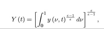
where y (ν, t) is the output level of intermediate ν at date t. The fact that many features of the model here are similar to the baseline endogenous technological change model highlights that the aggregate demand externalities that may lead to development traps here are already 887
present in our workhorse endogenous growth models. As usual ε is the elasticity of substitution between intermediate goods within a given period and is assumed to be strictly greater than one, i.e., ε > 1.
The production functions of intermediate goods in the two periods are as follows: 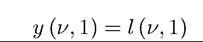 and
and 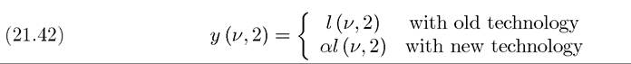 where a > 1 and l (ν, t) denotes labor devoted to the production of intermediate good ν at time t.
At date 1, there is a designated producer for each intermediate, but a competitive fringe can also enter and produce each good as productively as the designated producer. At date 1, the designated producer can also invest in the new technology, which costs F per firm. If this investment is undertaken, this producer’s productivity at date 2 will be higher by a factor α as indicated by equation (21.42). In contrast, the fringe will not benefit from this technological improvement, thus the designated producer will have some degree of monopoly power. The profits from intermediate producers are naturally allocated to the representative household.
Since this is a two-period economy, we will be looking for a subgame perfect equilibrium. Moreover, to simplify the discussion, let us focus on symmetric subgame perfect equilibria, SSPE. An SSPE consists of an allocation of labor across firms, investment decisions for firms, wages for both periods and an interest rate linking consumption between the two periods.
First, since all goods are symmetric, the first period labor market clearing is straightforward and we will have
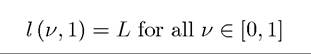
(recall that the measure of sectors and firms is normalized to 1). This implies that
At date 2, the equilibrium will depend on how many firms have adopted the new technology. Since we are looking at the symmetric equilibrium (SSPE), we only consider the two extremes where all firms adopt and no firm adopts. In either case, again the marginal productivity of all sectors are the same, so labor will be allocated equally, i.e.,
888
Consequently, when the technology is not adopted, we have
Y (2) = L
and when the technology is adopted by all the firms, we have
Y (2) = αL.
We now turn to the pricing decisions. In the first date, the designated producers have no monopoly power because of the competitive fringe, thus they charge price equal to marginal cost, which is w (1), and make zero profits. Since total output is equal to Y (1) = L, this also implies that the equilibrium wage rate is equal to
w (1) = 1.
In the second date, if the technology is not adopted, the same situation repeats, and we have w (2) = 1
and thus no profits. In this case there is also no investment, so consumption at both dates is equal to L, thus the interest rate that makes individuals happy to consume this amount in both periods is

To see this more formally, recall that the standard Euler equation in this case is  which can only be satisfied with C (1) = C (2), if the gross interest rate is R as given in
(21.44).
Next consider the situation in which the designated producers have invested in the advanced technology. Now they can produce α units of output with one unit of labor, while the fringe of competitive firms still produces one unit of output with one unit of labor. This implies that the designated producers have some monopoly power. The extent of this monopoly power depends on the comparison of ε and α.
Let us first determine the demand facing each producer, which is given as a solution to the following program of profit maximization for the final good sector:
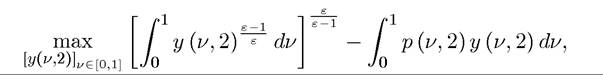
where p (ν, 2) is the price of intermediate ν at date 2. The first-order condition to this program implies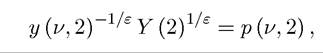
or 
This expression is useful in laying the foundations for the aggregate demand externalities, which we will discuss soon; the demand for intermediate ν depends on the total amount of production, Y (2).3 The familiar feature of the demand curve (21.46) is that it is iso-elastic.
To make further progress, first imagine the situation in which there is no fringe of competitive producers. In that case, each designated producer will act as an unconstrained monopolist and maximize its profits given by price minus marginal cost times quantity, i.e.,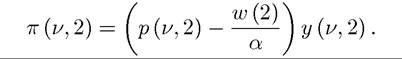
substituting from (21.46), the firm maximization problem is

which has a first-order condition
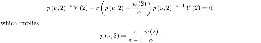
This is the standard monopoly price formula of a markup related to demand elasticity over the marginal cost, w (2) /α. Here the markup is constant because the demand elasticity is constant.
However, the monopolist can only charge this price if the competitive fringe could not enter and make profits stealing the entire market at this price. Since the competitive fringe can produce one unit using one unit of labor, the monopolist can only charge this price if ε/ ((ε — 1) α) ≤ 1. Otherwise, the price would be too high and the competitive fringe would enter. Let us assume that α is not so high as to make the monopolist unconstrained. In other words, we assume that
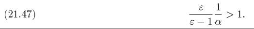
Under this assumption, the monopolist will be forced to charge a limit price. It is straightforward to see that this equilibrium limit price would be 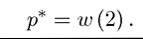
If it were any higher, the competitive fringe would enter, steal the whole market and make positive profits. If it were any lower, the monopolist could increase its price without losing
3
3The reader may wish to ask why there is an externality here.
Recall that even with perfectly competitive markets, the demand for goods supplied by a particular producer depends on the supply of other goods in the economy. So why is there an externality here? The answer, which may already be clear to some readers, will be discussed further below.the market, and thus increase its profits. This implies that under (21.47), each monopolist would make per unit profits equal to
The profits of firms are then obtained from substituting from (21.46) as:

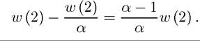
The wage rate can be determined from income accounting. Total production will be equal to Y (2) = αL, and this has to be distributed between profits and wages, thus 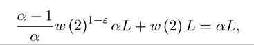 which has a solution of
as in the case without the technological investments. Therefore, in this economy the increased marginal product does not translate into higher wages. Instead, it leads to profits for firms. Nevertheless, all of these profits are redistributed to the agents, who are the owners of the firms. Thus C (2) = aL. However, because there was investment in the new technology at date 1, C (1) = L — F. Again the interest rate has to adjust so that individuals are happy to consume these amounts, i.e., so that they have a steep consumption profile without wanting to borrow. The Euler equation, (21.45), now implies
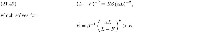
Consequently, the interest rate in this case is higher than the one in which there is no investment. This is natural, since investment implies that individuals are being asked to forgo date 1 consumption for date 2 consumption. Note also that the greater is θ, the higher is R, since with a greater θ, there is less intertemporal substitution. Also a higher F, meaning a greater consumption sacrifice at date 1 implies a higher interest rate.
The question is whether firms will find it profitable to undertake the investment at date 1. The reason for the possibility of multiplicity is that the answer to this question will depend on whether other firms are undertaking the investment or not. Let us first consider a situation in which no other firm is undertaking the investment, and consider the incentives of a single designated firm to undertake such an investment.
In this case total output at date 2 is equal to L (since the firm considering investment is infinitesimal), and the market interest rate is given by R. Moreover, from (21.48) and the 891
fact that w (2) = 1, profits at date 2 are
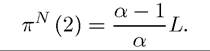
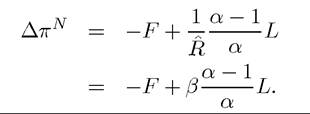
where the superscript N denotes that no other firm is undertaking the investment. Therefore, the net discounted profits at date 1 for the firm in question is
Next consider the case in which all other firms are undertaking the investment. In this case, profits at date 2 are
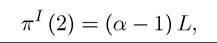
where the superscript I designates that all other firms are undertaking the investment. Consequently, the profit gain from investing at date 1 is
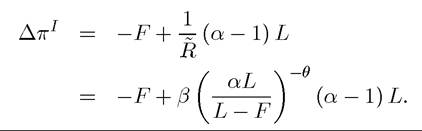
As discussed above, the idea of the paper by Murphy, Shleifer and Vishny (1989), similar to the ideas of many economists writing on economic development before them, was to generate multiple equilibria, where one of the equilibria corresponds to backwardness, while the other one corresponds to industrialization. In this context, this means that for the same parameter values both no investment in the new technology and all firms investing in the new technology should be equilibria. This is only possible if we have that is, when nobody else invests, investment is not profitable, and when all other firms invest, investment is profitable. This is clearly possible as of the aggregate demand externality ensures that π1 > πn; when other firms invest, they produce more, there is more aggregate demand, and therefore profits from having invested in the new technology are higher. Counteracting this effect is the fact that the interest rate is also higher when all firms invest. Therefore, the existence of multiple equilibria requires the interest rate effect not to be too strong. For example, in the extreme case where preferences are linear, i.e., θ = O, we have that


so (21.50) is certainly possible. More generally, the condition for the existence of multiple equilibria is that:
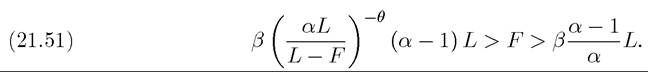
It is also straightforward to see that whenever both equilibria exist, the equilibrium with investment Pareto dominates the one without investment, since condition (21.51) implies that all households are better-off with the upward sloping consumption profile giving them higher consumption at date 2 (see Exercise 21.8). Therefore, this analysis establishes that when condition (21.51) is satisfied, there will exist two pure strategy SSPE. In one of these, all firms undertake the investment at date 1 and consumers are better off, while in the other one there are no investments in new technology and greater market failures. Intuitively, multiple equilibria emerge in this model because of aggregate demand externalities; investing in the new technology at date 1 is profitable only when there is sufficient demand at date 2 and there will be sufficient aggregate demand at date 2 when all firms invest in the new technology. This is at the root of the aggregate demand externalities, since the investment decision of a particular firm creates a positive (pecuniary) externality on other firms by increasing the level of demand facing their products. The reason why pecuniary externalities, which are present in all models, play a more important role here and lead to Pareto-ranked multiple equilibria is that each firm does not realize the full increase in the social product created by its investment, because the monopoly markup implies that at the margin further increases in output create a first-order gain for consumers. The presence of the markup means that the monopolist does not internalize this first-order gain, thus turning the demand linkages into aggregate demand externalities.
The interpretation for this result suggested by Murphy, Shleifer and Vishny is to consider the equilibrium with no investment in the new technology as representing a “development trap,” where the economy remains in “underdevelopment” because no firm undertakes the investment in new technology and this behavior implies that the demand necessary to make such investments profitable is absent. In contrast, the equilibrium with investment in new technology is interpreted as corresponding to “industrialization”. According to this interpretation, societies that can somehow coordinate on the equilibrium with investment (either because private expectations are aligned or because of some type of government action) will industrialize and realize both economic growth and Pareto improvement. As such, this model is argued to provide a formalization of the “big push” type industrialization described by economists such as Nurske or Rosenstein-Rodan. Although the idea of the big push and the aggregate demand externalities are attractive, the model here suffers from a number of obvious shortcomings. First, even though the process of industrialization is a dynamic one, the model here is static. Therefore, it does not allow a literal interpretation of a society being first in the no investment equilibrium and then changing to the investment equilibrium and industrializing. Second, as already discussed in Chapter 4, models with multiple equilibria do not provide a satisfactory model of development, since it is difficult to imagine a society remaining unable to coordinate on a simple range of actions that would make all
households (and firms) better off. Instead, it is much more likely that the ideas related to aggregate demand externalities (or other potential forces leading to multiple equilibria) are more important as sources of persistence or as mechanisms generating multiple steady states (while still maintaining a unique equilibrium path). In the next section, we will discuss how certain factors can lead to multiple steady states in dynamic models instead of the multiple equilibria emphasized by Murphy, Shleifer and Vishny in the context of a static model. I will illustrate these issues focusing on another set of topics that appear to be important in the context of development, the interaction between the distribution of income and human capital investments.
21.6.
More on the topic Multiple Equilibria From Aggregate Demand Externalities and the Big Push:
- Inequality, Credit Market Imperfections and Human Capital
- Contents
- Acemoglu D.. Introduction to Modern Economic Growth. Princeton University Press,2008. — 1248 p., 2008
- Table of contents
- Agricultural Productivity and Industrialization