Innovation by Incumbents and Entrants and Sources of Productivity Growth
A key aspect of the growth process is the interplay between innovations and productivity improvements by existing firms on the one hand and entry by more productive, new firms on the other.
The evidence from industry studies, which will be discussed in greater detail in Section 18.1, suggests that a large part of productivity growth at the industry level (and thus in the aggregate) comes from productivity improvements by continuing plants, though entry by new plants also makes a nontrivial contribution to industry productivity growth. The Schumpeterian models presented in this section have emphasized entry by new firms as the engine of growth. Interpreted literally, these models predict that all growth should be driven by entry, which is at odds with the facts. The expanding variety models presented in the previous chapter also do not provide a framework for the analysis of the interplay between existing firms and new entrants.[20] In this and the next section, I discuss models that feature productivity growth by continuing plants (firms). The model in this section will feature productivity growth both by incumbents and entrants. The model in the next section will be richer in many respects, but will not allow entry. The two models together provide a first glimpse of the types of models that might be useful for studying the industrial organization of innovation and productivity growth.14.3.1. Model. The economy is again in continuous time and admits a representative household with the standard CRRA preferences, as in (13.1) in the previous chapter. Population is constant at L and labor is supplied inelastically. The resource constraint at time t takes the usual form
 where C (t) is consumption, X (t) is aggregate spending on machines, and Z (t) is total expenditure on R&D at time t.
The production function of the unique final good is given by

where x(ν, t | q) is the quantity of the machine of type ν of quality q used in the production process and the measure of machines is again normalized to 1. This aggregate production function is very similar to (14.3) used above, except that the quality of machines comes in with an exponent β. This has no effects on any of the results concerning growth, but will imply that firms with different productivity levels will have different levels of sales (see Exercise 14.27). It will therefore enable us to make predictions about the size distribution of firms as well.
The engine of economic growth is again quality improvements, but these will be driven by two types of innovations:
(1) Innovation by incumbents
(2) Creative destruction by entrants.
Let q (ν, t) be the quality of machine line ν at time t. Consider the following “quality ladder” for each machine type:

where λ > 1 and n (ν, t) denotes the number of incremental innovations on this machine line between time s ≤ t and time t, where time s is the date at which this particular type of technology was first invented and q (ν, s) refers to its quality at that point. The incumbent has a fully enforced patent on the machines that it has developed (though this patent does not prevent entrants leapfrogging the incumbent’s machine quality). I assume that at time t = 0, each machine line starts with some quality q (ν, 0) > 0 owned by an incumbent with fully enforce patent on this initial machine quality. Incremental innovations can only be performed by the incumbent producer. So we can think of those as “tinkering” innovations that improve the quality of the machine. The assumption that incumbents have access to a technology to create incremental innovations is consistent with case study evidence (e.g., Freemen, 1982, or Sherer, 1984).
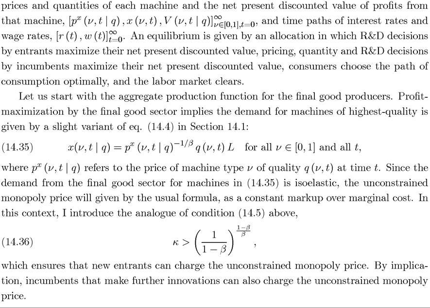
14.3.2. Equilibrium. Since the demand for machines in (14.35) is isoelastic and ψ ? 1 — β, the profit-maximizing monopoly price is
id="Picutre 1590" class="lazyload" data-src="/files/uch_group77/uch_pgroup317/uch_uch7365/image/image1589.jpg">
Combining this with (14.35) implies that

Consequently, the flow profits of a firm with the monopoly rights on the machine of quality q can be computed as:

Next, substituting (14.38) into (14.31), total output is given by an expression identical to (14.8) above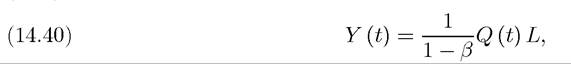
with average quality of machines Q (t) given as in (14.9) in Section 14.1. Aggregate spending on machines is

Moreover, since the labor market is competitive, the wage rate at any point in time is given by (14.11) as before.
To characterize the full equilibrium, we need to determine R&D effort levels by incumbents and entrants. To do this, let us write the net present value of a monopolist with the highest quality of machine q at time t in machine line ν. This value satisfies the standard Hamilton-Jacobi-Bellman equation
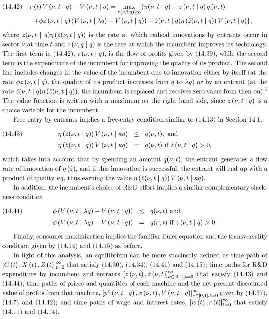
5The fact that the incumbent receives a zero value from then on follows from the assumption that a previous incumbent has no advantage relative to other entrants in competing for another round of innovations.
in view of the first inequality (14.55).
(4) The transversality condition: condition (14.15) should hold so that the maximization problem of the representative household is well-defined. The condition r* > g* is necessary and sufficient to ensure (14.15). The second inequality in (14.55) ensures that this inequality holds.
Therefore, the BGP is interior and is uniquely defined.
I next prove that the BGP also gives the unique dynamic equilibrium path. Let us start with two observations.
z(ν,t | q) = z* for all ν, q and t, (14.60) implies that V (ν,t | q) is linear in q in this case as well.
Finally, the result that surviving firms expand on average and that all firms die with probability 1 follows from eq. (14.57). ?
Proposition 14.6 focuses on equilibria in which all incumbents exert the same R&D effort. Exercise 14.26 shows that the same conclusions hold when we do not focus on such equilibria.
14.3.3. Some Numbers. I will now try to flesh out the implications of this model on the decomposition of productivity growth between incumbents and entrants. Although some of the parameters of the current model are difficult to pin down with our current knowledge of the technology of R&D, some simple back-of-the-envelope calculations are still informative. Let us choose the following standard numbers:

where the last number, the intertemporal elasticity of substitution, is pinned down by the choice of the other three numbers. The first three numbers refer to annual rates (implicitly defining ∆t = 1 as one year). There is much greater uncertainty concerning the remaining parameters. Let us normalize φ = L = 1. For the rest, I will report a number of different possibilities.
As a benchmark, As a benchmark, I take β = 2/3, which implies that two thirds of national income accrues to labor and one third to profits. The requirement in (14.36) then implies that ę > 1.7. I also take the benchmark value of κ = 3, so that entry by new firms is sufficiently “radical” as suggested by some of the qualitative accounts of the innovation process (e.g., Freeman, 1982, Scherer, 1984). Innovation by incumbents is taken to be correspondingly smaller λ = 1.2. This implies that productivity gains from a radical innovation is about ten times that of a standard “incremental” innovation by incumbents (i.e., (κ — 1) / (λ — 1) = 10). I will then show how the results change when the magnitudes of radical and incremental innovations are varied. For the function η (z), I adopt the following frequently-used form: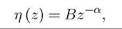
and choose the benchmark value of α = 0.5. The remaining two parameters, φ and B will be chosen to ensure g* = 0.02. I start with the benchmark value of φ = 0.4, but this value will need to be modified in some of the variations in order to satisfy condition (14.55) above or to ensure g* = 0.02. With these numbers, (14.48) implies
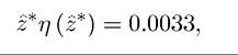
and
The value for also implies that there is entry of a new firm (creative destruction) in each machine line on average once every 7.5 years (recall that r* = 0.05 as the annual interest 534

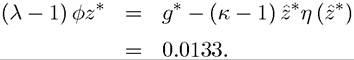
Therefore, in this benchmark parameterization, over two thirds of productivity growth comes from innovation by incumbents.
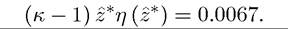
Moreover, φz* = 0.0667, so that there are on average 1.2 incremental innovations per year by an incumbent in a particular machine line (r*∕φz* ≈ 1.2). Using alternative values of the parameters κ, λ, β and α leads to broadly similar conclusions, though depending on the exact parameterization the contribution of entrants to productivity growth can be larger or smaller.14.3.4. The Effects of Policy on Growth. Let us now use this model to analyze the effects of policies on equilibrium productivity growth and its decomposition between incumbents and entrants. Since the model has a Schumpeterian structure (with quality improvements as the engine of growth and creative destruction playing a major role), it may be conjectured that entry barriers (or taxes on potential entrance) will have negative effects on economic growth as in the baseline model earlier in this chapter. To investigate whether this is the case, let us suppose that there is a tax τe on R&D expenditure by entrants and a tax τi on R&D expenditure by incumbents (naturally, these can be taken to be negative and interpreted as subsidies as well). Note also that the tax on entrants, τe, can be interpreted as a more strict patent policy than the one in the baseline model, where the entrant did not have to pay the incumbent for partially benefiting from its accumulated knowledge. Nevertheless, to keep the analysis brief, I only focus on the case in which tax revenues are collected by the government rather than rebated back to the incumbent as patent fees.
Repeating the analysis above yields the following equilibrium conditions:

The equation that determines the optimal R&D decisions of incumbents, (14.45), is also modified because of the tax rate τi and becomes

Now combining (14.61) with (14.62),

Consequently, the BGP R&D level by entrants z*, when their R&D is taxed at the rate τe, is given by
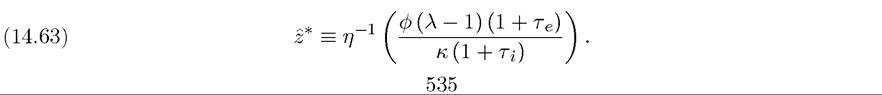
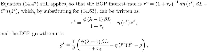
with Z* given by (14.63). The following is now immediate:
The result in this proposition is rather surprising and extreme. As shown above, in Schumpeterian models, making entry more difficult, either with entry barriers or by taxing R&D by entrants, has negative effects on economic growth. Despite the Schumpeterian nature of the current model, here blocking entry increases equilibrium growth. Moreover, as Exercise 14.24 shows, in the decentralized equilibrium of this economy there tends to be too much entry, so a tax on entry also tends to improve welfare. The intuition for this result is related to the main departure of this model from the standard Schumpeterian models. In contrast to the baseline Schumpeterian models, the engine of growth is still quality improvements, but these are undertaken both by incumbents and entrants. Entry barriers, by protecting incumbents, increase their value and greater value by incumbents encourages more R&D investments and faster productivity growth. Taxing entrants makes incumbents more profitable and this encourages further innovation by the incumbents. Taxes on entrants or entry barriers also further increase the contribution of incumbents to productivity growth.
Nevertheless, the result in this proposition should be interpreted with caution. The model in this section is special in that the R&D technology of incumbents is a linear. This linearity is important for the results in Proposition 14.7. Exercise 14.26 shows that the equilibrium can be characterized even when φ (z) is a concave function of z, and in this case, the effect of taxes on entrants is ambiguous, because it encourages R&D by incumbents and discourages R&D by entrants. Therefore, Proposition 14.7 should be read as emphasizing a particular new channel in the stark as possible way, not as a realistic description of how innovation will respond to tax policies.
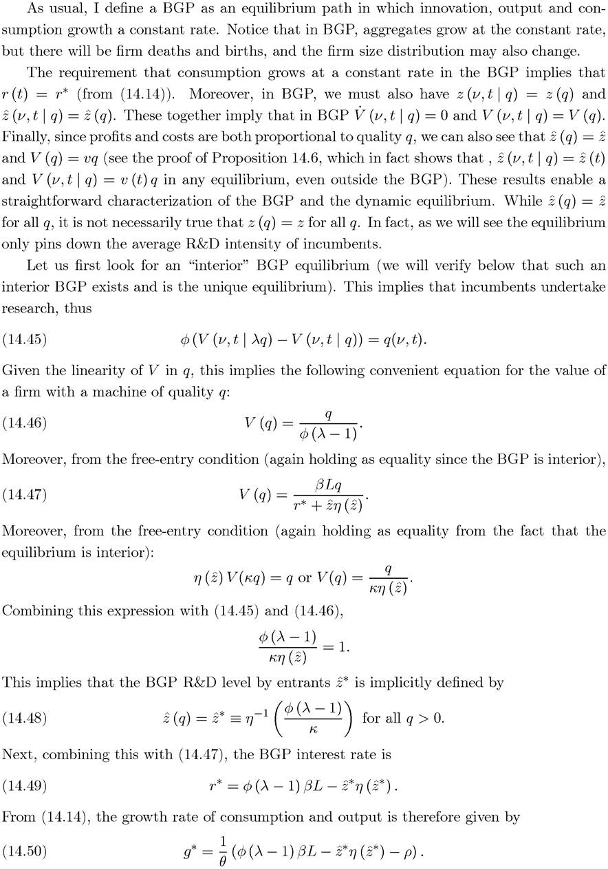
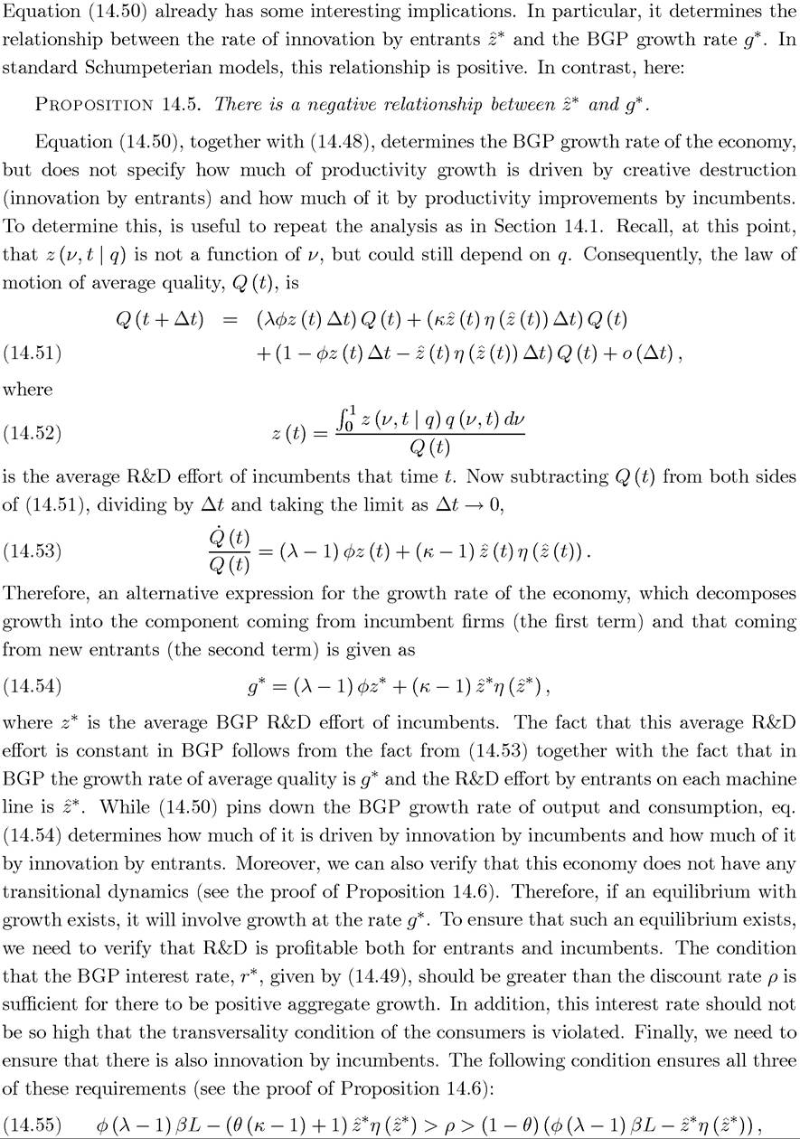
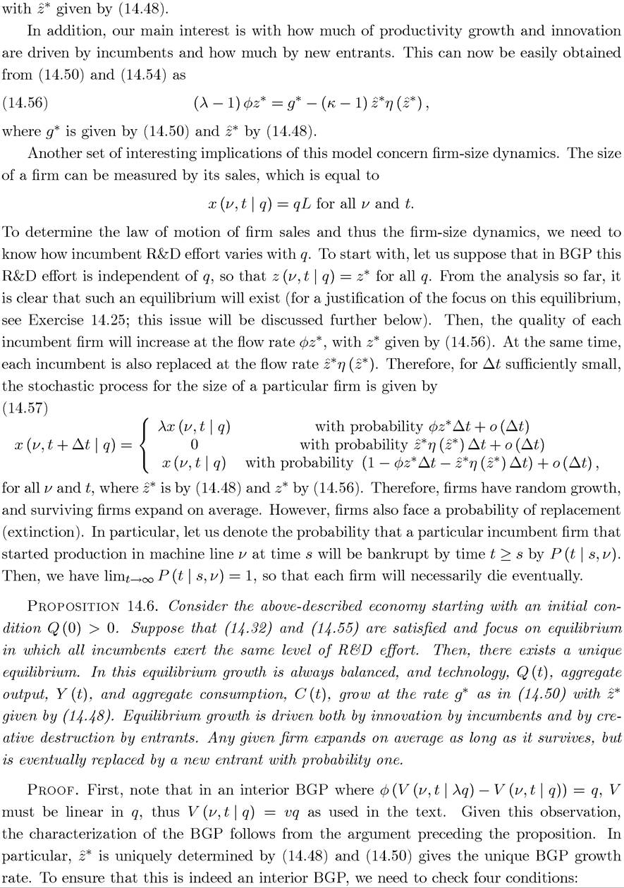
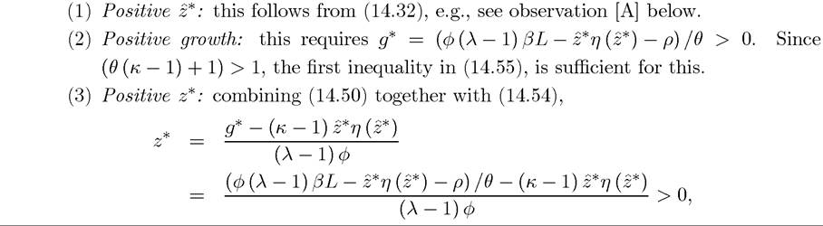
14.4.