Step-by-Step Innovations*
In the baseline Schumpeterian model and also in the extended Schumpeterian model of the previous section, new entrants could undertake innovation on any machine and did not need to have developed any knowhow on a particular line of business.
This led to a simple structure, in many ways parallel to the models of expanding varieties studied in the previous chapter. However, quality improvements in practice may have a ma jor cumulative 536 aspect. For example, it may be that only firms that have already reached a certain level of knowledge in a particular product or machine line can engage in further innovations. This is in fact consistent with qualitative accounts of technological change and competition in specific industries. Abernathy (1980, p. 70), for instance, concludes his study of a number of diverse industries by stating that: “each of the major companies seems to have made more frequent contributions in a particular area,” and argues that this is because previous innovations in a field facilitate future innovations. This aspect is entirely missing from the baseline model of Schumpeterian growth, where any firm can engage in research to develop the next higher- quality machine (and in addition Arrow’s replacement effect implies that incumbents do not undertake R&D, though this aspect was relaxed and generalized in the previous section). A more realistic description of the research process may involve only a few firms engaging in continuous and cumulative innovation, and in competition in a particular product or machine line.This section presents a model of cumulative innovation of this type. Following Aghion, Harris, Howitt and Vickers (2001), we will refer to this as a model of step-by-step innovation. Such models are not only useful in providing a different conceptualization of the process of Schumpeterian growth, but they also enable us to endogenize the equilibrium market structure and allow a richer analysis of the effects of competition and intellectual property rights policy.
Together with the model of innovation by incumbents and entrants presented in the previous section, this model enables us to have a framework in which existing firm (continuing establishments) contribute to productivity growth and build on their own past innovations (consistent with the empirical evidence as discussed in Section 18.1 in Chapter 18). In fact, the model in this section has a number of distinctive features relative to those presented so far in this and the previous chapter. For instance, these models predict that weaker patent protection and greater competition should reduce economic growth. Nevertheless, existing empirical evidence suggests that typically industries that are more competitive experience faster growth (or at the very least, there is a non-monotonic relationship between competition and economic growth, see, for example, Blundell (1999), Nickell (1999) and Aghion, Bloom, Blundell, Griffith and Howitt (2005)). Schumpeterian models with an endogenous market structure show that the effects of competition and intellectual property rights on economic growth are more complex, and greater competition (and weaker intellectual property rights protection) sometimes increases the growth rate of the economy.14.4.1. Preferences and Technology. Consider the following continuous-time economy with a unique final good. The economy is populated by a continuum of measure 1 of individuals, each with 1 unit of labor endowment, which they supply inelastically. To simplify the analysis, I assume that the instantaneous utility function takes a logarithmic form. Thus the representative household has preferences given by
Let Y (t) be the total production of the final good at time t. The economy is closed and the final good is used only for consumption (there is no investment or spending on machines), so that C (t) = Y (t). The standard Euler equation from (14.64) then implies that

where this equation defines g (t) as the growth rate of consumption and thus output, and r (t) is the interest rate at date t.
The final good Y is produced using a continuum 1 of intermediate goods according to the Cobb-Douglas production function

where y (ν,t) is the output of νth intermediate at time t. Throughout, I take the price of the final good (or the ideal price index of the intermediates) as the numeraire and denote the price of intermediate ν at time t by py (ν, t). I also assume that there is free entry into the final good sector. These assumptions, together with the Cobb-Douglas production function (14.66), imply that each final good producer will have the following demand for intermediates
id="Picutre 1618" class="lazyload" data-src="/files/uch_group77/uch_pgroup317/uch_uch7365/image/image1617.jpg">
Intermediate ν ∈ [0,1] come in two different varieties, each produced by one of two infinitely-lived firms. These two varieties are perfect substitutes and compete a la Bertrand. No other firm is able to produce in this industry. Firm i = 1 or 2 in industry ν has the following technology

where li (ν, t) is the employment level of the firm and qi (ν, t) is its level of technology at time t. The only difference between the two firms is their technology, which will be determined endogenously. As in the models studied so far, each consumer in the economy holds a balanced portfolio of the shares of all firms. Consequently, the objective function of each firm is to maximize expected profits.
The production function for intermediate goods, (14.68), implies that the marginal cost of producing intermediate ν for firm i at time t is

where w (t) is the wage rate in the economy at time t.
Let us denote the technological leader in each industry by i and the follower by —i, so that:
Bertrand competition between the two firms implies that all intermediates will be supplied by the leader at the limit price (see Exercise 14.28):

Equation (14.67) then implies the following demand for intermediates:

R&D by the leader or the follower stochastically leads to innovation.
We assume that when the leader innovates, its technology improves by a factor λ > 1. The follower, on the other hand, can undertake R&D to catch up with the frontier technology. Let us assume that because this innovation is for the follower’s variant of the product and results from its own R&D efforts, it does not constitute infringement of the patent of the leader, and the followerdoes not have to make any payments to the technological leader in the industry.
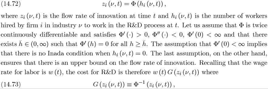
R&D investments by the leader and the follower may have different costs and success probabilities. Nevertheless, I simplify the analysis here by assuming that they have the same costs and the same probability of success. In particular, in all cases, each firm (in every industry) has access to the following R&D technology (innovation possibilities frontier):
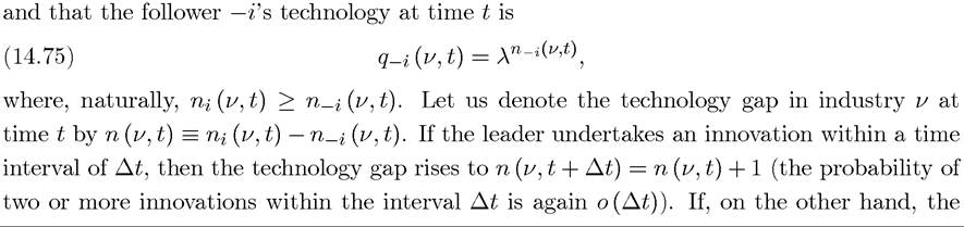
follower undertakes an innovation during the interval ∆t, then n (ν,t + ∆t) = 0. In addition, let us assume that there is an intellectual property rights (IPR) policy of the following form: the patent held by the technological leader expires at the exponential rate ę < ∞, in which case, the follower can close the technology gap.
Given this specification, the law of motion of the technology gap in industry ν can be
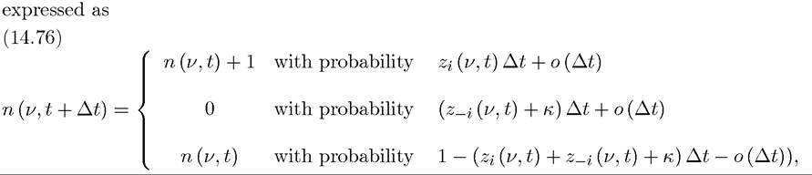
where o (∆t) again represents second-order terms, in particular, the probabilities of more than one innovations within an interval of length ∆t. The terms Zi (ν, t) and z-i (ν, t) are the flow rates of innovation by the leader and the follower, while κ is the flow rate at which the follower is allowed to copy the technology of the leader.
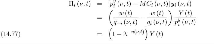
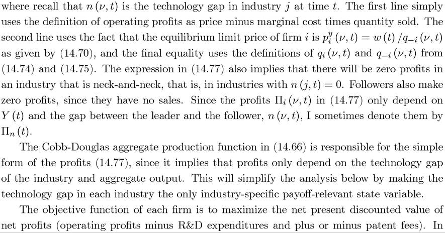
In the first line, when n (ν, t) = 0, so that the two firms are neck-and-neck, zi (ν,t) should be taken as equal to 2z (ν,t), since the two firms will undertake the same amount of research effort given by z (ν, t) and the technology gap will increase to 1 if one of them is successful, which has probability 2z (ν,t).We next write the instantaneous “operating” profits for the leader (the profits exclusive of R&D expenditures and license fees). Profits of leader i in industry ν at time t are
In addition, there is demand for labor coming from R&D of both followers and leaders in all industries. Using (14.72) and the definition of the G function, we can express industry demands for R&D labor as
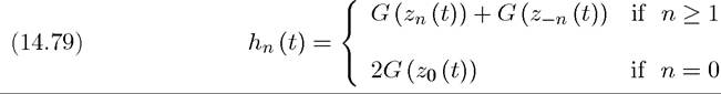
where z-n (t) refers to the R&D effort of a follower that is n steps behind. Moreover, this expression takes into account that in an industry with neck-and-neck competition, i.e., with n = 0, there will be twice the demand for R&D coming from the two “symmetric” firms.
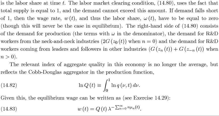
The labor market clearing condition can then be expressed as:
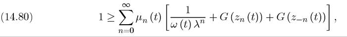
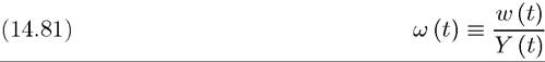
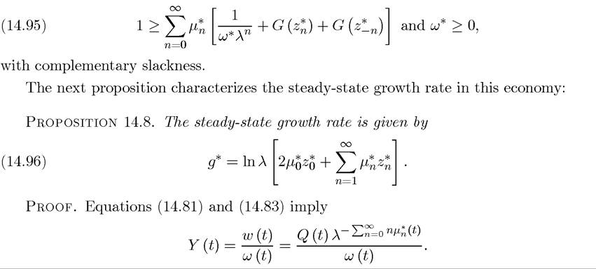
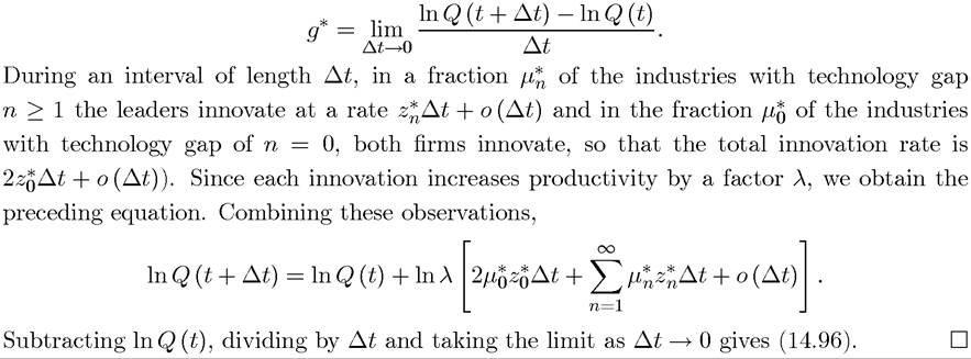
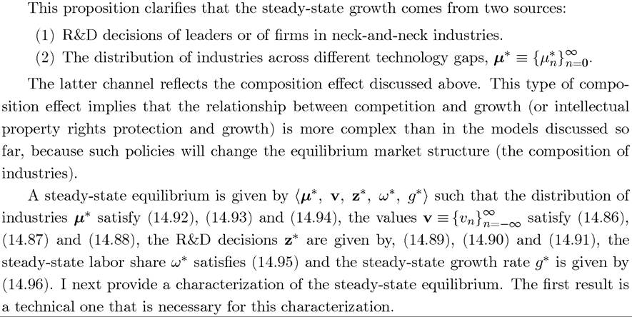
and ω (t) ≥ 0, with complementary slackness, where
14.4.3.
Steady-State Equilibrium. Let us now focus on steady-state (Markov Per-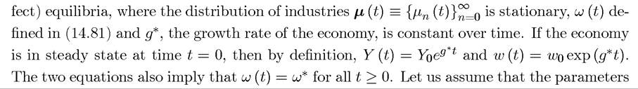 are such that the steady-state growth rate g* is positive, but not large enough to violate the transversality conditions. This implies that net present values of each firm at all points in time will be finite and enable us to write the maximization problem of a leader that is n > 0 steps ahead recursively.

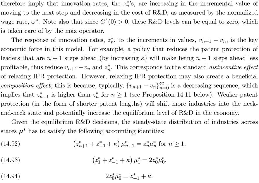
The first expression equates exit from state n + 1 (which takes the form of the leader going one more step ahead or the follower catching-up the leader) to entry into this state (which takes the form of a leader from the state n making one more innovation). The second equation, (14.93), performs the same accounting for state 1, taking into account that entry into this state comes from innovation by either of the two firms that are competing neck-and-neck. Finally, eq. (14.94) equates exit from state 0 with entry into this state, which comes from innovation by a follower in any industry with n ≥ 1.
The labor market clearing condition in steady state can then be written as


 ?
?
This proposition therefore shows that the highest amount of R&D is undertaken in neck- and-neck industries. This explains why composition effects can increase aggregate innovation. Exercise 14.32 shows how a relaxation of intellectual property rights protection can increase the growth rate in the economy.
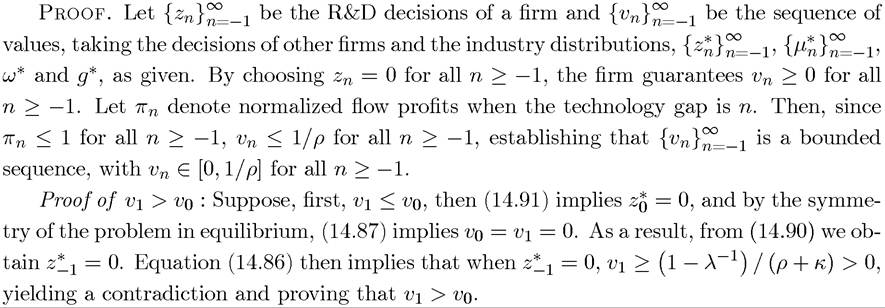
So far, I have not provided a closed-form solution for the growth rate in this economy. It turns out that this is generally not possible, because of the endogenous market structure in these types of models. Nevertheless, it can be proved that a steady-state equilibrium exists in this economy, though the proof is somewhat more involved and does not generate additional insights for our purposes (see Acemoglu and Akcigit, 2006).
An important feature of this model is that equilibrium markups are endogenous and evolve over time as a function of competition between the firms producing in the same product line. More importantly, Proposition 14.11 implies that when a particular firm is sufficiently ahead of its rival, it undertakes less R&D. Therefore, this model, contrary to the baseline Schumpeterian model and also contrary to all expanding varieties models, implies that greater competition may lead to higher growth rates. Greater competition generated by closing the gap between the followers and leaders induces the leaders to undertake more R&D in order to escape the competition from the followers.
14.5.