Key Facts about Aggregate Fluctuations

Historically, the process of economic growth has been anything but smooth. As can be seen from both figures 1.2 and 1.3, GDP per capita displays significant fluctuations around its long-run trend.

In accounting for the key facts about aggregate fluctuations, I present evidence mainly from the United States and the United Kingdom. These two countries have long and relatively consistent time series for the relevant variables, and, to a large extent, it is the experience of these two countries that has contributed to the development of macroeconomics as we know it. However, where appropriate, I present evidence for other countries as well.³¹

1.3.1 Frequency, Severity, and Duration of Recessions

Figure 1.4 presents the evolution of the log of real GDP per capita in the United States from 1854 to 2014. Figure 1.5 shows the evolution of the log of real GDP per capita in the United Kingdom from 1820 to 2014. The gray shaded areas indicate years of recession. Recessions are generally defined as periods in which there is a contraction in economic activity, with real GDP falling rather than rising.

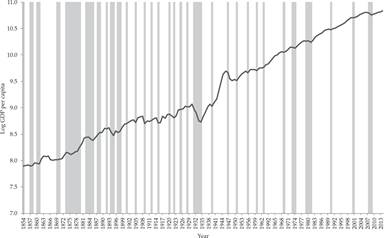
Figure 1.4 Recessions (shaded areas) and (log) per capita GDP in the United States.

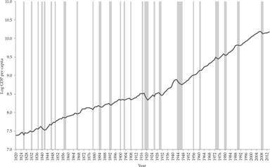
Figure 1.5 Recessions (shaded areas) and (log) per capita GDP in the United Kingdom.

In the United States, the Business Cycle Dating Committee of the National Bureau of Economic Research (NBER) is generally considered to be the authority for dating US recessions. The NBER defines an economic recession as “a significant decline in economic activity spread across the economy, lasting more than a few months, normally visible in real GDP, real income, employment, industrial production, and wholesale-retail sales (nber.org/cycles).” In the United Kingdom, recessions are generally defined as two consecutive quarters of negative economic growth, as measured by the seasonally adjusted quarter-on-quarter figures for real GDP.

As can be seen from figure 1.4, there were 54 years of recession in the United States between 1854 and 2014, and 107 years of no recession. In periods of recession, per capita GDP usually falls or remains stagnant. In the 161 years between 1854 and 2014, a recession occurred, on average, in 1 out of every 3 years. After World War II, a drop in the frequency of US recessions occurred. There were 14 years of recession between 1946 and 2014. In the 69 postwar years, a recession occurred, on average, in 1 out of every 4.9 years.

In the United Kingdom (figure 1.5), there were 41 years of recession between 1820 and 2014, and 154 years of no recession. In the 195 years between 1820 and 2014, a recession occurred on average in 1 out of every 4.75 years. In the post–World War II period, there were 13 years of recession, with a recession occurring in 1 out of every 5.3 years on average.

What is also clear from figures 1.4 and 1.5 is that not all recessions are alike. Many recessions are short and shallow, but a few deep and quite prolonged ones also occur.

The longest US recession was that of the 1870s, while the deepest and second-longest recession was the Great Depression of the 1930s. The recessions of the 1890s were the deepest recessions before the onset of the Great Depression. In the post–World War II period, the most severe recessions were the ones of the early 1970s and early 1980s, as well as the recent recession of 2008–2009. In the United Kingdom, deep and long recessions occurred in the 1840s, in the aftermath of the two World Wars, in the early and late 1970s and the early 1980s, in the early 1990s, as well as in 2008–2009.³²

1.3.2 Unemployment in Booms and Recessions

One of the key characteristics of recessions is that they are associated with falls in employment and persistent rises in unemployment rates.³³

Figures 1.6 and 1.7 depict the evolution of unemployment rates in the United States and the United Kingdom, respectively.

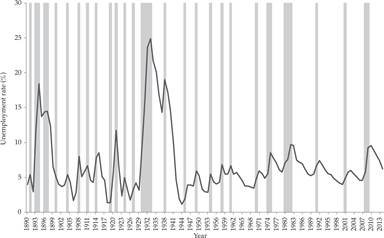
Figure 1.6 Recessions (shaded areas) and the unemployment rate in the United States.

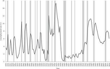
Figure 1.7 Recessions (shaded areas) and the unemployment rate in the United Kingdom.

The rise in unemployment is considered by many as the most significant economic and social cost of recessions, along with the general fall in real incomes.

Whereas in the pre–World War II period, unemployment in the United States tended to fluctuate around a rate slightly below 5% of the labor force, during the Great Depression, unemployment reached almost 25% of the labor force. The average unemployment rate in the 1930s was 18.8% of the US labor force, higher than the peak unemployment rate of 18.4% in the previously deepest recession of the 1890s.³⁴

In the post–World War II period, fluctuations in the US unemployment rate are smaller but significant nonetheless. In the recession of the 1970s, unemployment rose from 4.9% of the labor force in 1973 to a peak of 8.5% in 1975. In the recession of the early 1980s, unemployment rose from 5.8% of the labor force in 1979 to 9.7% in 1982. In the recession of 2008–2009, unemployment rose from 4.6% of the labor force in 2007 to 9.6% in 2010.

The UK experience is not too different. Unemployment rates as high as 7–10% were not uncommon in the recessions of the nineteenth century. In the recession of the early 1920s, unemployment rose to 12.1%, and in the Great Depression of the early 1930s, it rose to a peak of 15.3% in 1932.

In the post–World War II period unemployment in the United Kingdom was remarkably low for many years.

The sustained and persistent rise in unemployment, along with the sustained drop in real incomes, is thus one of the key characteristics of recessions, and one of the most important reasons that macroeconomics is concerned with aggregate fluctuations. Unemployment not only rises during recessions, but it also persists, and on many occasions, it peaks after a recession has turned into recovery. Thereafter, it falls only gradually during the recovery.

1.3.3 Trends and Fluctuations in the Price Level and Inflation

A third key macroeconomic variable that concerns both the general public and policymakers is the price level, and its rate of change, the rate of inflation. The price level and its rate of change is what determines the purchasing power of money incomes. Figures 1.8 and 1.9 depict the evolution of the price level in the United States and the United Kingdom, respectively, as measured by the index of consumer prices, while figures 1.10 and 1.11 depict the evolution of inflation.

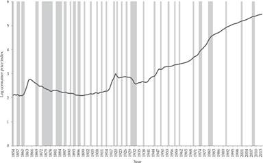
Figure 1.8 Evolution of the price level in the United States (shaded areas indicate recessions).

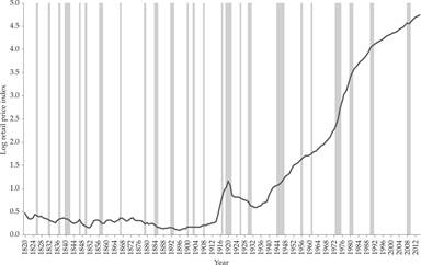
Figure 1.9 Evolution of the price level in the United Kingdom (shaded areas indicate recessions).

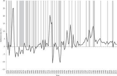
Figure 1.10 Evolution of consumer price index(CPI) inflation in the United States (shaded areas indicate recessions).

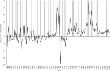
Figure 1.11 Evolution of CPI inflation in the United Kingdom (shaded areas indicate recessions).

Some interesting facts emerge from these figures with regard to the evolution of the price level and inflation.

The first fact is that before World War II, the price level did not display a marked upward trend, as it did after World War II. If anything, there were long periods of a falling price level, both during the gold standard period and in the interwar years. Inflation was a temporary phenomenon, associated with wars, such as the American Civil War of 1861–1865, World War I, or periods of economic boom. In contrast, the price level tended to fall during recessions, which were thus also periods of deflation.

Average annual inflation during 1854–1913 was only 0.6% in the United States, and average annual inflation during 1821–1913 in the United Kingdom was negative, −0.2% (figures 1.10 and 1.11). The price level in the United Kingdom was on a slightly negative trend until World War I. Had it not been for the American Civil War, the United States would probably also have been characterized by falling prices.

During the American Civil War, US inflation averaged approximately 15% per year, with peak inflation rates of about 25% in both 1863 and 1864. During World War I, average annual inflation was equal to 9.7% in the United States and to 15.3% in the United Kingdom.

During the interwar period (1919–1939), deflation occurred in both countries. Prices in the United States were falling by 0.2% per year on average, whereas prices in the United Kingdom were falling by 0.9% per year on average.

As can be seen from figures 1.8–1.11, after World War II, the price level displays a significant positive trend in both the United States and the United Kingdom. Average inflation has been positive and periodically high in both countries throughout the post–World War II period.

In addition, the negative impact of recessions on the price level and inflation, which was a regular characteristic of the pre–World War II period, does not seem to hold as firmly in the postwar period. The recessions of the 1970s and the early 1980s are associated with an increase rather than a decrease in inflation, a phenomenon that has been described as stagflation.

What stands out when trying to explain the long-run trends of the price level and inflation is (1) the very high correlation of inflation and the rate of growth of the money supply and (2) the total lack of correlation of economic growth and the growth of the money supply.

Figure 1.12 shows the close correlation between inflation and the rate of growth of the money supply, as measured by a broad measure of the money stock (M2) in 110 countries, for 1960–1990. The correlation coefficient is equal to 0.95. In figure 1.13, one can see the complete absence of any correlation between the growth rate of real GDP and the rate of growth of the money supply. The correlation coefficient is −0.014 and is not statistically significant.

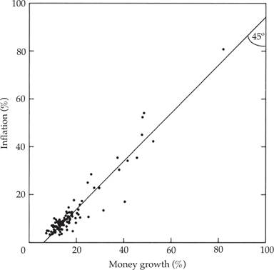
Figure 1.12 Money growth and inflation in 110 countries, 1960–1990. Adapted from McCandles and Weber [1995].

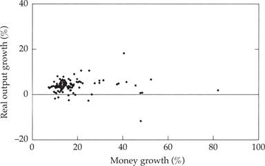
Figure 1.13 Money growth and real GDP growth in 110 countries, 1960–1990. Adapted from McCandles and Weber [1995].

These two facts—the almost complete correlation of money growth and inflation and the total absence of any correlation between money growth and economic growth—form the empirical basis of the assumption of the long-run neutrality of money, characteristic of both models of economic growth and models of aggregate fluctuations. This long-run neutrality of money is one of the main predictions of the quantity theory of money. As Lucas [1996, p. 668] has commented:

The prediction that prices respond proportionally to changes in money in the long run, deduced by Hume in 1752 (and by many other theorists, by many different routes, since), has received ample—I would say decisive—confirmation, in data from many times and places. The observation that money changes induce output changes in the same direction receives confirmation in some data sets but is hard to see in others. Large-scale reductions in money growth can be associated with large-scale depressions or, if carried out in the form of a credible reform, with no depression at all.

As we shall see when we discuss models of the determination of inflation in the relevant chapters 7, 12, and 20, one cannot explain the evolution of the price level and inflation without reference to monetary policy and its relation to fiscal policy and the aims of stabilization policy.

1.3.4 Monetary Policy and Government Debt

At the risk of running a bit ahead of our discussion in the relevant chapter, I provide a short explanation of the trends in prices and inflation depicted in figures 1.8–1.11. A fuller explanation will have to wait for the analysis of models of inflation and monetary policy in chapters 7, 12, and 20, and the determination of fiscal policy and government debt in chapters 6 and 21.

There was no systematic inflation and the price level did not display a particular trend until World War I, because for most of this period, both the United States and the United Kingdom had adopted metallic monetary systems, based on precious metals (specie), such as gold and silver. Such metallic systems constrained the rate of growth of the money supply. When they were forced to temporarily abandon such systems, as during wars, both countries sought to return to such systems as soon as possible.

Britain had been on a de facto gold standard since the early eighteenth century. The United States had been on a silver standard until 1834, on a bimetallic standard until 1861, and on an effective gold standard since 1879.

During the Napoleonic Wars of 1803–1815 in the United Kingdom and the American Civil War of 1861–1865 in the United States, the convertibility to specie was suspended. Thus, the link of the money supply to gold and silver was relaxed through the issuance of nonconvertible paper currency. The Bank of England issued nonconvertible sterling banknotes, and the United States issued nonconvertible greenbacks. The issuance of nonconvertible banknotes was used to finance these countries’ respective war and resulted in large increases in the money supply. The increase in the money supply resulted in a rise in the price level through inflation. Yet in both countries, the suspension of convertibility was always considered to be temporary. Sterling convertibility was restored in 1821, and dollar convertibility was finally restored in 1879.

What happened during the Napoleonic Wars and the American Civil War is an example of the use of seigniorage (i.e., revenue from money creation) to partly finance temporary increases in government expenditure. Government expenditure rises significantly during a war, and money creation is one of the ways to finance this temporarily increased expenditure. The other is government debt.

Figure 1.14 depicts the federal debt of the US government as a percentage of GDP since 1792. With a few exceptions, episodes of significant increase in the ratio of federal debt to GDP are associated with recessions and major wars, such as the American Civil War and the two great wars of the twentieth century (during 1914–1918 and 1939–1945). Major recessions, such as the Great Depression of the early 1930s and the Great Recession of 2008–2009, are also associated with significant hikes in government debt.

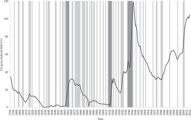
Figure 1.14 Evolution of US federal debt as a percentage of GDP (dark shaded areas indicate major wars; light shaded areas indicate recessions).

Wars require significant rises in government expenditure. Governments, instead of raising taxes, resort to temporary borrowing and inflationary finance to minimize the economic and political disadvantages of significant hikes in taxes. The same happens during recessions. Recessions result in a temporary fall in tax revenues, because of the reduction in economic activity, and temporary increases in expenditure on unemployment insurance and social protection.

Hence, both wars and recessions result in rises in government deficits and debts and, in the case of wars, they result in increases in revenue from money creation. We shall examine the relationship between war finance, inflation, and government debt in various parts of the book (mainly in chapters 12 and 21).

The United States had remained on the gold standard during World War I. In addition, in 1913, the Federal Reserve System was created and assumed the role of the central bank of the United States. The money supply increased less in the United States than in the United Kingdom during World War I, as the war affected the US economy and federal government expenditure less than in the case of Britain. As a result, the need for seigniorage was not as large in the United States.

Figure 1.15 depicts UK public debt as a percentage of GDP since 1792. Significant rises in the ratio of British public debt to GDP are associated with major wars, such as the Napoleonic Wars (1803–1815) and the two great wars of the twentieth century. As in the case of the United States, they are also associated with recessions, such as the Great Depression of the early 1930s and the Great Recession of 2008–2009.

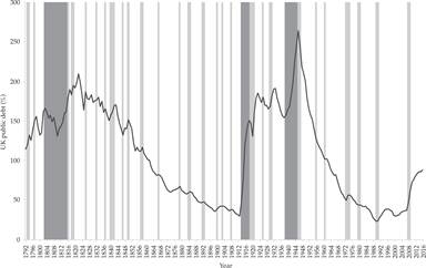
Figure 1.15 Evolution of UK public debt as a percentage of GDP (dark shaded areas indicate major wars; light shaded areas indicate recessions).

During World War I, the United Kingdom resorted to both government debt and money creation when convertibility to gold was suspended. The reason was again to help finance the war without disruptive rises in taxes.

However, after the war, the major aim of UK postwar financial policy became the return to gold at the prewar parity. Thus, from the early 1920s, UK monetary policy was extremely deflationary so as to reverse the wartime rise of the price level and allow sterling to return to the gold standard at the prewar parity to gold and the US dollar.

The 1920s was a period of monetary instability for many European economies. Germany, and other economies in Central Europe, experienced hyper inflations that totally disrupted their payments system. The underlying cause was the need to pay war reparations and the excessive use of seigniorage (see chapter 12).

The United Kingdom returned to the gold standard in 1925, after a prolonged period of deflation. However, when the Great Depression struck, the United Kingdom was forced to again abandon the gold standard, which it duly did in 1931. The United States, which had maintained the gold standard during the war, also allowed the dollar to be gradually devalued by about 40% against gold in both 1933 and 1934. From $20.67 an ounce, the price of gold rose to $35 an ounce.

The gold standard changed permanently in 1934, as gold coinage was discontinued in the United States, and significant holdings of gold coins or bullion by the public were made illegal. Thus, convertibility only remained for the purposes of foreign payments. This change had important consequences for monetary policy and inflation, especially in the post–World War II period.

To explain the change in the behavior of prices and inflation during World War II and especially in the postwar period, one must thus again refer to monetary policy. Both the United States and the United Kingdom resorted to significant increases in the money supply to finance part of the cost of World War II. As a result, the price level and inflation rose, despite extensive price controls during the war.

1.3.5 Monetary Policy and Inflation in the Postwar Period

The nature of monetary policy changed after World War II. The Bretton Woods system of fixed but adjustable exchange rates, which was agreed upon in 1944 by the United States, the United Kingdom, and a host of other countries, was quite different from the international gold standard. Although the United States undertook to maintain a fixed price of gold at $35 an ounce and managed to do so until 1968, convertibility existed only among central banks, and for the purpose of foreign payments. Domestic convertibility to gold was not restored in any of the industrial economies. The United Kingdom and other industrial economies undertook to maintain a fixed exchange rate vis-à-vis the dollar, but the system allowed for currency devaluations in the case of “fundamental disequilibrium.”

Monetary policy in the post–World War II period, free from the constraints of convertibility and influenced by Keynesian macroeconomics, was directed toward the goal of maintaining high employment. This was partly because no country was prepared to see a return to the unemployment rates of the 1930s.

As we shall see in the relevant chapters (chapters 15 and 20), if a central bank seeks to keep unemployment at a very low rate, it can eventually lead to high inflation through an increase in inflationary expectations. Until the 1980s, the Federal Reserve, the Bank of England, and other central banks sought to maintain low nominal interest rates. The money supply accommodated changes in the demand for money, caused either by real output growth or by inflation. The goal of maintaining low unemployment took higher precedence relative to the prewar period, which contributed to a rise in the average rate of inflation.

When the Bretton Woods system collapsed in the early 1970s, monetary policy became even more conducive to inflation. Inflation, which until the late 1960s was persistently positive but relatively low, increased significantly in the 1970s, a period also characterized by two recessions and low growth. As mentioned earlier, the term stagflation was invented to explain this phenomenon. It was only after the restrictive monetary policies of the early 1980s in the United States, the United Kingdom, and other industrial economies, that inflation returned to low levels, as their monetary authorities changed the primary emphasis of monetary policy from low unemployment to low inflation.

To summarize, neither the long-run evolution nor the fluctuations of the price level and inflation can be analyzed without reference to monetary and fiscal factors and policies. In periods of temporarily high government expenditure, such as wars, monetary policy is subordinated to fiscal policy, as governments finance a large part of the increased expenditure through money creation and government debt. Money creation results in inflation, which is higher during wars.

In the period before World War II, when most developed countries were on the gold or silver standard, their price levels did not display a significant upward trend, and average inflation was close to zero. This was because the requirement of convertibility constrained the rate of growth of the money supply to be very low. Periods of war often resulted in suspension of convertibility and temporarily high inflation, as monetary policy was subordinated to the financing needs of national treasuries, and so the rate of growth of the money supply increased significantly. Periods of recession were usually associated with deflation and moderate increases in government debt.

In the post–World War II period, the stance of monetary policy appears to have become more accommodative, leading to a positive trend for the price level and permanently positive inflation. Inflation increased significantly in the 1970s, when the system of floating exchange rates further freed up national monetary policies to pursue high employment targets.

Since the early 1980s, the problem of high inflation has been addressed in the main industrial economies, as national central banks shifted the focus of monetary policy from low unemployment to low inflation. The negative link between inflation and recessions was also broken in the post–World War II period, as the recessions of the 1970s were characterized by rises in inflation, resulting in stagflation.

But some countries continue to be plagued by high inflation rates. The underlying reason for their problems is the same as that which caused inflation to rise in wartime in both the United States and the United Kingdom. This is none other than the need to finance part of government expenditure through seigniorage, as other methods of finance do not suffice. Thus, the problem of high and persistent inflation in some countries (or even the problem of hyperinflation) has its roots in the inadequacies of those countries’ fiscal systems, or their temporary collapse because of wars, civil wars, revolutions, or extreme forms of political and economic instability. Models that can explain episodes of very high inflation and hyperinflation are analyzed in chapter 12.

1.4