Long-Run Growth: The Solow Model
Explain the factors affecting long-run living standards in the Solow model.
In this section we take a closer look at the dynamics of economic growth, or how the growth process evolves over time.
In doing so, we drop the assumption made in Chapter 3 that the capital stock is fixed and study the factors that cause the economy's stock of capital to grow. Our analysis is based on a famous model of economic growth developed in the late 1950s by Nobel laureate Robert Solow[99] of MIT, a model that has become the basic framework for most subsequent research on growth. Besides clarifying how capital accumulation and economic growth are interrelated, the Solow model is useful for examining two basic questions about growth:1. What is the relationship between a nation's long-run standard of living and fundamental factors such as its saving rate, its population growth rate, and its rate of technical progress?
2. How does a nation's rate of economic growth evolve over time? Will economic growth stabilize, accelerate, or stop?
Setup of the Solow Model
The Solow model examines an economy as it evolves over time. To analyze the effects of labor force growth as well as changes in capital, we assume that the population is growing and that at any particular time a fixed share of the population is of working age. For any year, t,
Nt = the number of workers available.
We assume that the population and work force both grow at fixed rate n. So, if n = 0.01, the number of workers in any year is 1% greater than in the previous year.
At the beginning of each year, t, the economy has available a capital stock, Kt. (We demonstrate shortly how this capital stock is determined.) During each year, t, capital, Kt, and labor, Nt, are used to produce the economy's total output, Yt.
Part of the output produced each year is invested in new capital or in replacing worn-out capital. We further assume that the economy is closed and that there are no government purchases,[100] so the uninvested part of output is consumed by the population. IfYt = output produced in year t,
It = gross (total) investment in year t, and
Ct = consumption in year t,
the relationship among consumption, output, and investment in each year is
Ct = Yt - It. (6.4)
Equation (6.4) states that the uninvested part of the economy's output is consumed.
Because the population and the labor force are growing in this economy, focusing on output, consumption, and the capital stock per worker is convenient. Hence we use the following notation:
The capital stock per worker, kt, is also called the capital-labor ratio. An important goal of the model is to understand how output per worker, consumption per worker, and the capital-labor ratio change over time.[101]
The Per-Worker Production Function. In general, the amount of output that can be produced by specific quantities of inputs is determined by the production function. Until now we have written the production function as a relationship between total output, Y, and the total quantities of capital and labor inputs, K and N. However, we can also write the production function in per-worker terms as
yt = f (kt). (6.5)
Equation (6.5) indicates that, in each year t, output per worker, yt, depends on the amount of available capital per worker, kt.[102] Here we use a lower case f instead of an upper case F for the production function to emphasize that the measurement of output and capital is in per-worker terms. For the time being we focus on the role of the capital stock in the growth process by assuming no productivity growth and thus leaving the productivity term out of the production function, Eq.
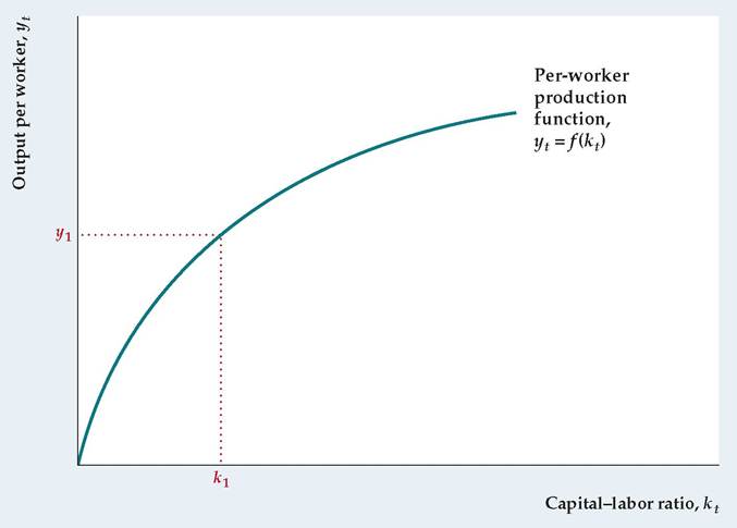
(6.5).[103] We bring productivity growth back into the model later.The per-worker production function is graphed in Figure 6.3. The capitallabor ratio (the amount of capital per worker), kt, is measured on the horizontal axis, and output per worker, yt, is measured on the vertical axis. The production function slopes upward from left to right because an increase in the amount of capital per worker allows each worker to produce more output. As with the standard production function, the bowed shape of the per-worker production function reflects the diminishing marginal productivity of capital. Thus when the capitallabor ratio is already high, an increase in the capital-labor ratio has a relatively small effect on output per worker.
FIGURE 6.3
The per-worker production function
The per-worker production function, yt = f (kt), relates the amount of output produced per worker, yt, to the capital-labor ratio, kt. For example, when the capital-labor ratio is k 1, output per worker is y1. The per-worker production function slopes upward from left to right because an increase in the capital-labor ratio raises the amount of output produced per worker. The bowed shape of the production function reflects the diminishing marginal productivity of capital.
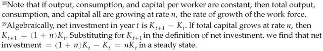
Steady States. One of the most striking conclusions obtained from the Solow model is that in the absence of productivity growth the economy reaches a steady state in the long run. A steady state is a situation in which the economy's output per worker, consumption per worker, and capital stock per worker are constant— that is, in the steady state, yt, ct, and kt don't change over time.18 To explain how the Solow model works, we first examine the characteristics of a steady state and then discuss how the economy might attain it.
Let's begin by looking at investment in a steady state. In general, gross (total) investment in year t, It, is devoted to two purposes: (1) replacing worn-out or depreciated capital, and (2) expanding the size of the capital stock. If d is the capital depreciation rate, or the fraction of capital that wears out each year, the total amount of depreciation in year t is dKt. The amount by which the capital stock is increased is net investment. What is net investment in a steady state? Because capital per worker, KJNt, is constant in a steady state, the total capital stock grows at the same rate as the labor force—that is, at rate n. Net investment is therefore nKt in a steady state.19 To obtain steady-state gross investment, we add steady-state net investment nKt and depreciation dKt:
It =( n + d) Kt (in a steady state).
(6.6)
To obtain steady-state consumption (output less investment), we substitute Eq. (6.6) into Eq. (6.4):

Equation (6.7) measures consumption, output, and capital as economywide totals rather than in per-worker terms. To put them in per-worker terms, we divide both sides of Eq. (6.7) by the number of workers, Nt, recalling that ct = CJNt, yt = YJNt, and kt = KJNt. Then we use the per-worker production function, Eq. (6.5), to replace yt with f (kt) and obtain

Equation (6.8) shows the relationship between consumption per worker, c, and the capital-labor ratio, k, in the steady state. Because consumption per worker and the capital-labor ratio are constant in the steady state, we dropped the time subscripts, t.
Equation (6.8) shows that an increase in the steady-state capital-labor ratio, k, has two opposing effects on steady-state consumption per worker, c. First, an increase in the steady-state capital-labor ratio raises the amount of output each worker can produce, f (k). Second, an increase in the steady-state capital-labor ratio increases the amount of output per worker that must be devoted to investment, (n + d) k. More goods devoted to investment leaves fewer goods to consume.
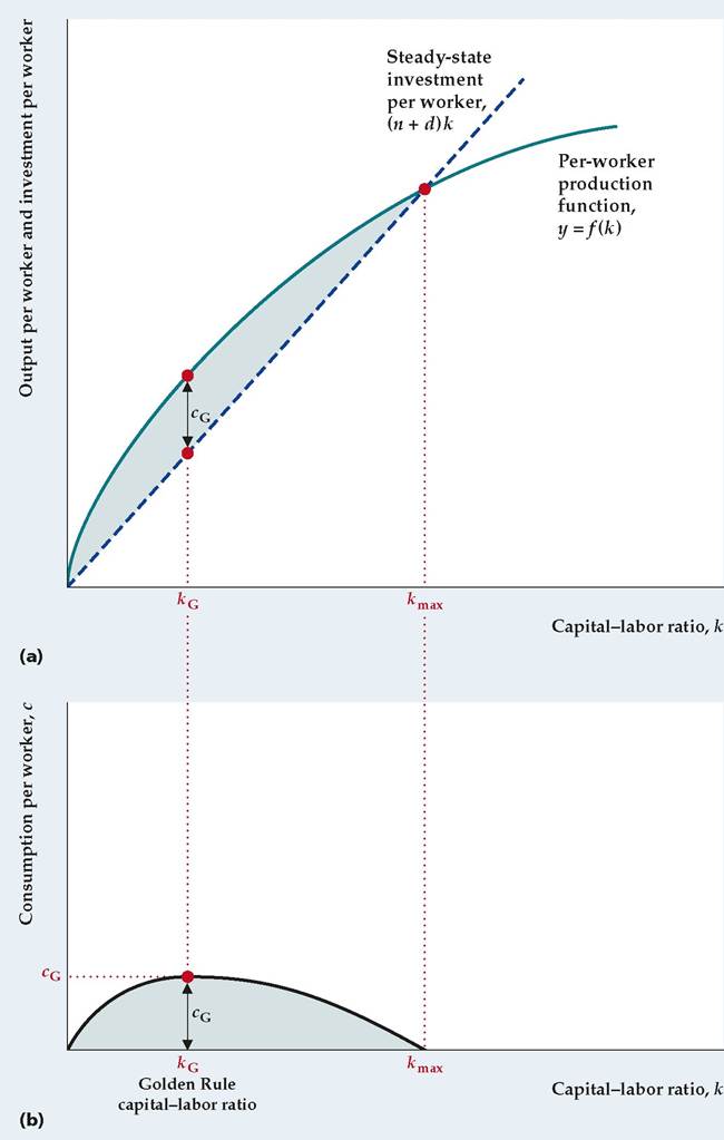
Figure 6.4 shows the trade-off between these two effects. In Fig. 6.4(a) different possible values of the steady-state capital-labor ratio, k, are measured on the horizontal axis. The curve is the per-worker production function, y = f (k), as in Fig. 6.3. The straight line shows steady-state investment per worker, (n + d) k. Equation (6.8) indicates that steady-state consumption per worker, c, equals the height of the curve, f (k), minus the height of the straight line, (n + d) k. Thus consumption per worker is the height of the shaded area.
The relationship between consumption per worker and the capital-labor ratio in the steady state is shown more explicitly in Fig. 6.4(b). For each value of the steady-state capital-labor ratio, k, steady-state consumption, c, is the difference between the production function and investment in Fig. 6.4(a). Note that, starting from low and medium values of k (values less than kG in Fig. 6.4(b)), increases in the steady-state capital-labor ratio lead to greater steady-state consumption per worker. The level of the capital-labor ratio that maximizes consumption per worker in the steady state, shown as kG in Fig. 6.4, is known as the Golden Rule capital-labor ratio, so-called because it maximizes the economic welfare of future generations.[104]
However, for high values of k (values greater than the Golden Rule capitallabor ratio, kG), increases in the steady-state capital-labor ratio actually result in lower steady-state consumption per worker because so much investment is needed to maintain the high level of capital per worker.
In the extreme case, where k = k max in Fig. 6.4, all output has to be devoted to replacing and expanding the capital stock, with nothing left to consume!Policymakers often try to improve long-run living standards with policies aimed at increasing the capital-labor ratio by stimulating saving and investment. Figure 6.4 shows the limits to this strategy. A country with a low amount of capital per worker may hope to improve long-run (steady-state) living standards
FIGURE 6.4
The relationship of consumption per worker to the capital-labor ratio in the steady state
(a) For each value of the capital-labor ratio, k, steady-state output per worker, y, is given by the per-worker production function, f (k). Steadystate investment per worker, (n + d )k, is a straight line with slope
n + d. Steady-state consumption per worker, c, is the difference between output per worker and investment per worker (the shaded area). For example, if the capitallabor ratio is kG, steadystate consumption per worker is cG. (b) For each value of the steady-state capital-labor ratio, k, steady-state consumption per worker, c, is derived in (a) as the difference between output per worker and investment per worker. Thus the shaded area in
(b) corresponds to the shaded area in (a). Note that, starting from a low value of the capital-labor ratio, an increase in the capital-labor ratio raises steady-state consumption per worker. However, starting from a capitallabor ratio greater than the Golden Rule level, kG, an increase in the capitallabor ratio actually lowers consumption per worker. When the capital-labor ratio equals k max, all output is devoted to investment, and steady-state consumption per worker is zero. further. Indeed, Fig. 6.4 shows that, theoretically, capital per worker can be so high that further increases will actually lower steady-state consumption per worker.
substantially by increasing its capital-labor ratio. However, a country that already has a high level of capital per worker may find that further increases in the capitallabor ratio fail to raise steady-state consumption much. The fundamental reason for this outcome is the diminishing marginal productivity of capital—that is, the larger the capital stock already is, the smaller the benefit from expanding the capital stock
In any economy in the world, could a higher capital stock lead to less consumption in the long run? An empirical study of seven advanced industrial countries concluded that the answer is "no." Even for high-saving Germany, further increases in capital per worker would lead to higher steady-state consumption per worker.[105] Thus in our analysis we will always assume that an increase in the steady-state capital-labor ratio raises steady-state consumption per worker.
Reaching the Steady State. Our discussion of steady states leaves two loose ends. First, we need to say something about why an economy like the one we describe here eventually will reach a steady state, as we claimed earlier. Second, we have not yet shown which steady state the economy will reach; that is, we would like to know the steady-state level of consumption per worker and the steady-state capital-labor ratio that the economy will eventually attain.
To tie up these loose ends, we need one more piece of information: the rate at which people save. To keep things as simple as possible, suppose that saving in this economy is proportional to current income:
St = sYt, (6.9)
where St is national saving[106] in year t and s is the saving rate, which we assume to be constant. Because a $1 increase in current income raises saving, but by less than $1 (see Chapter 4), we take s to be a number between 0 and 1. Equation (6.9) ignores some other determinants of saving discussed in earlier chapters, such as the real interest rate. However, including these other factors wouldn't change our basic conclusions, so for simplicity we omit them.
In every year, national saving, St, equals investment, It. Therefore
sYt = (n + d)Kt (in a steady state), (6.10)
where the left side of Eq. (6.10) is saving (see Eq. 6.9) and the right side of Eq. (6.10) is steady-state investment (see Eq. 6.6).
Equation (6.10) shows the relation between total output, Yt, and the total capital stock, Kt, that holds in the steady state. To determine steady-state capital per worker, we divide both sides of Eq. (6.10) by Nt. We then use the production function, Eq. (6.5), to replace yt with f (kt):
sf (k) = (n + d)k (in the steady state). (6.11)
Equation (6.11) indicates that saving per worker, sf (k), equals steady-state investment per worker, (n + d) k. Because the capital-labor ratio, k, is constant in the steady state, we again drop the subscripts, t, from the equation.
With Eq. (6.11) we can now determine the steady-state capital-labor ratio that the economy will attain, as shown in Figure 6.5. The capital-labor ratio is measured along the horizontal axis. Saving per worker and investment per worker are measured on the vertical axis.
FIGURE 6.5
Determining the capital-labor ratio in the steady state
The steady-state capitallabor ratio, k*, is determined by the condition that saving per worker, sf (k), equals steadystate investment per worker, (n + d )k. The steady-state capital-labor ratio, k*, corresponds to point A, where the saving curve and the steadystate investment line cross. From any starting point, eventually the capital-labor ratio reaches k *. If the capital-labor ratio happens to be below k * (say, at k 1), saving per worker, sf (k1), exceeds the investment per worker, (n + d )k 1, needed to maintain the capital-labor ratio at k 1. As this extra saving is converted into capital, the capital-labor ratio will rise, as indicated by the arrows. Similarly, if the capital-labor ratio is greater than k * (say, at k 2), saving is too low to maintain the capitallabor ratio, and the capital-labor ratio will fall over time.
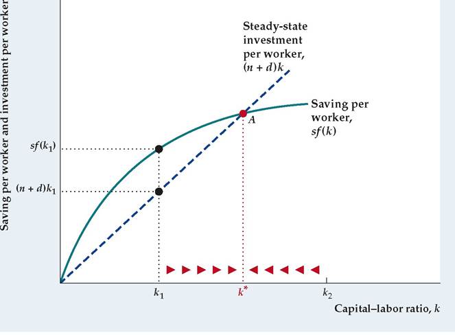
The bowed curve shows how the amount of saving per worker, sf (k), is related to the capital-labor ratio. This curve slopes upward because an increase in the capital-labor ratio implies higher output per worker and thus more saving per worker. The saving-per-worker curve has the same general shape as the perworker production function, because saving per worker equals the per-worker production function, f (k), multiplied by the fixed saving rate, s.
The line in Fig. 6.5 represents steady-state investment per worker, (n + d) k. The steady-state investment line slopes upward because, as the capital-labor ratio rises, more investment per worker is required to replace depreciating capital and equip new workers with the same high level of capital.
According to Eq. (6.11), the steady-state capital-labor ratio must ensure that saving per worker and steady-state investment per worker are equal. The one level of the capital-labor ratio for which this condition is satisfied is shown in Fig. 6.5 as k*, the value of k at which the saving curve and the steady-state investment line cross. For any other value of k, saving and steady-state investment won't be equal. Thus k * is the only possible steady-state capital-labor ratio for this economy.[107]
With the unique steady-state capital-labor ratio, k*, we can also find steadystate output and consumption per worker. From the per-worker production function, Eq. (6.5), if the steady-state capital-labor ratio is k*, steady-state output per worker, y*, is
y* = f (k*).
From Eq. (6.8) steady-state consumption per worker, c*, equals steady-state output per worker, f (k *), minus steady-state investment per worker, (n + d) k *:
c* = f (k*) — (n + d) k*.
Recall that, in the empirically realistic case, a higher value of the steady-state capital-labor ratio, k*, implies greater steady-state consumption per worker, c*.
Using the condition that in a steady state, national saving equals steady-state investment, we found the steady-state capital-labor ratio, k *. When capital per worker is k*, the amount that people choose to save will just equal the amount of investment necessary to keep capital per worker at k *. Thus, when the economy's capital-labor ratio reaches k*, it will remain there forever.
But is there any reason to believe that the capital-labor ratio will ever reach k * if it starts at some other value? Yes, there is. Suppose that the capital-labor ratio happens to be less than k *; for example, it equals k 1 in Fig. 6.5. When capital per worker is k 1, the amount of saving per worker, sf (k 1), is greater than the amount of investment needed to keep the capital-labor ratio constant, (n + d) k 1. When this extra saving is invested to create new capital, the capital-labor ratio will rise. As indicated by the arrows on the horizontal axis, the capital-labor ratio will increase from k 1 toward k *.
If capital per worker is initially greater than k*—for example, if k equals k2 in Fig. 6.5—the explanation of why the economy converges to a steady state is similar. If the capital-labor ratio exceeds k*, the amount of saving that is done will be less than the amount of investment that is necessary to keep the capital-labor ratio constant. (In Fig. 6.5, when k equals k2, the saving curve lies below the steady-state investment line.) Thus the capital-labor ratio will fall over time from k 2 toward k*, as indicated by the arrows. Output per worker will also fall until it reaches its steady-state value.
To summarize, if we assume no productivity growth, the economy must eventually reach a steady state. In this steady state the capital-labor ratio, output per worker, and consumption per worker remain constant over time. (However, total capital, output, and consumption grow at rate n, the rate of growth of the labor force.) This conclusion might seem gloomy because it implies that living standards must eventually stop improving. However, that conclusion can be avoided if, in fact, productivity continually increases.
The Fundamental Determinants of Long-Run Living Standards
What determines how well off the average person in an economy will be in the long run? If we measure long-run well-being by the steady-state level of consumption per worker, we can use the Solow model to answer this question (keeping in mind that we are assuming that an increase in the steady-state capital-labor ratio will increase steady-state consumption per worker). Here, we discuss three factors that affect long-run living standards: the saving rate, population growth, and productivity growth (see Summary table 8).
The Saving Rate. According to the Solow model, a higher saving rate implies higher living standards in the long run, as illustrated in Figure 6.6. Suppose that the economy's initial saving rate is s1 so that saving per worker is s1 f (k). The saving curve when the saving rate is s1 is labeled "Initial saving per worker." The initial steady-state capital-labor ratio, k *, is the capital-labor ratio at which the initial saving curve and the investment line cross (point A).
SUMMARY 8
The Fundamental Determinants of Long-Run Living Standards
| An increase in | Causes long-run output, consumption, and capital per worker to | Reason |
| The saving rate, s | Rise | Higher saving allows for more investment and a larger capital stock. |
| The rate of population growth, n | Fall | With higher population growth more output must be used to equip new workers with capital, leaving less output available for consumption or to increase capital per worker. |
| Productivity | Rise | Higher productivity directly increases output; by raising incomes, it also raises saving and the capital stock. |
Suppose now that the government introduces policies that strengthen the incentives for saving, causing the country's saving rate to rise from s1 to s2. The increased saving rate raises saving at every level of the capital-labor ratio. Graphically, the saving curve shifts upward from s1 f (k) to s 2 f (k). The new steadystate capital-labor ratio, k 2, corresponds to the intersection of the new saving curve and the investment line (point B). Because k 2 is larger than k *, the higher saving rate has increased the steady-state capital-labor ratio. Gradually, this economy will move to the higher steady-state capital-labor ratio, as indicated by the arrows on the horizontal axis. In the new steady state, output per worker and consumption per worker will be higher than in the original steady state.
FIGURE 6.6
The effect of an increased saving rate on the steady-state capital-labor ratio An increase in the saving rate from s1 to s2 raises the saving curve from s1 f (k) to s2 f (k). The point where saving per worker equals steadystate investment per worker moves from point A to point B, and the corresponding capitallabor ratio rises from k* to k *. Thus a higher saving rate raises the steady-state capital-labor ratio.
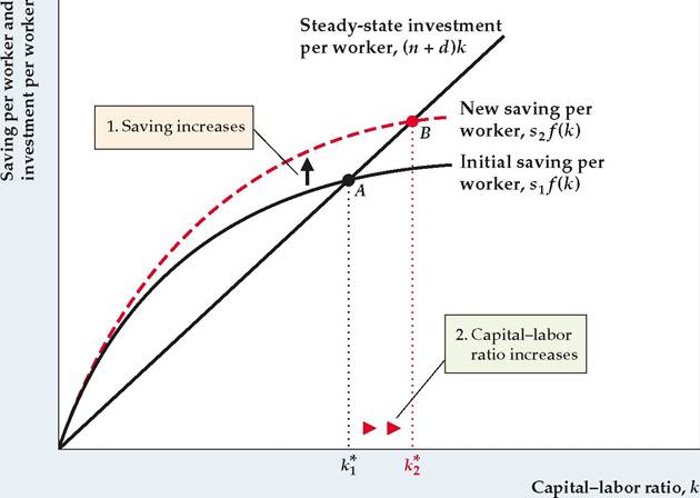
FIGURE 6.7
The effect of a higher population growth rate on the steady-state capital-labor ratio An increase in the population growth rate from n1 to n2 increases steadystate investment per worker from (n1 + d )k to (n2 + d)k. The steadystate investment line pivots up and to the left as its slope rises from n1 + d to n2 + d. The point where saving per worker equals steadystate investment per worker shifts from point A to point B, and the corresponding capital-labor ratio falls from k* to k *. A higher population growth rate therefore causes the steady-state capital-labor ratio to fall.
An increased saving rate leads to higher output, consumption, and capital per worker in the long run, so it might seem that a policy goal should be to make the country's saving rate as high as possible. However, this conclusion isn't necessarily correct: Although a higher saving rate raises consumption per worker in the long run, an increase in the saving rate initially causes consumption to fall. This decline occurs because, at the initial level of output, increases in saving and investment leave less available for current consumption. Thus higher future consumption has a cost in terms of lower present consumption. Society's choice of a saving rate should take into account this trade-off between current and future consumption. Beyond a certain point the cost of reduced consumption today will outweigh the long-run benefits of a higher saving rate.
Population Growth. In many developing countries a high rate of population growth is considered a major problem, and reducing it is a primary policy goal. What is the relationship between population growth and a country's level of development, as measured by output, consumption, and capital per worker?
The Solow model's answer to this question is shown in Figure 6.7. An initial steady-state capital-labor ratio, k *, corresponds to the intersection of the steadystate investment line and the saving curve at point A. Now suppose that the rate of population growth, which is the same as the rate of labor force growth, rises from an initial level of n1 to n 2. What happens?
An increase in the population growth rate means that workers are entering the labor force more rapidly than before. These new workers must be equipped with capital. Thus, to maintain the same steady-state capital-labor ratio, the amount of investment per current member of the work force must rise. Algebraically, the rise in n increases steady-state investment per worker from (n1 + d) k to (n 2 + d) k. This increase in the population growth rate causes the steady-state investment line to pivot up and to the left, as its slope rises from (n1 + d) to (n 2 + d).
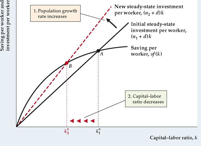
After the pivot of the steady-state investment line, the new steady state is at point B. The new steady-state capital-labor ratio is k2, which is lower than the original capital-labor ratio, k*. Because the new steady-state capital-labor ratio is lower, the new steady-state output per worker and consumption per worker will be lower as well.
Thus the Solow model implies that increased population growth will lower living standards. The basic problem is that when the work force is growing rapidly, a large part of current output must be devoted just to providing capital for the new workers to use. This result suggests that policies to limit population growth will indeed improve living standards.
There are some counterarguments to the conclusion that policy should aim to reduce population growth. First, although a reduction in the rate of population growth n raises consumption per worker, it also reduces the growth rate of total output and consumption, which grow at rate n in the steady state. Having fewer people means more for each person but also less total productive capacity. For some purposes (military, political) a country may care about its total output as well as output per person. Thus, for example, some European countries are concerned about projections that their populations will actually shrink in the coming decades, possibly reducing their ability to defend themselves or influence world events.
Second, an assumption in the Solow model is that the proportion of the total population that is of working age is fixed. When the population growth rate changes dramatically, this assumption may not hold. For example, declining birth rates in the United States imply that the ratio of working-age people to retirees will decline in the twenty-first century, a development that may cause problems for Social Security funding and other areas such as health care.
Productivity Growth. A significant aspect of the basic Solow model is that, ultimately, the economy reaches a steady state in which output per capita is constant. But in the introduction to this chapter we described how Japanese output per person has grown by a factor of about 30 since 1870! How can the Solow model account for that sustained growth? The key is a factor that we haven't yet made part of the analysis: productivity growth.
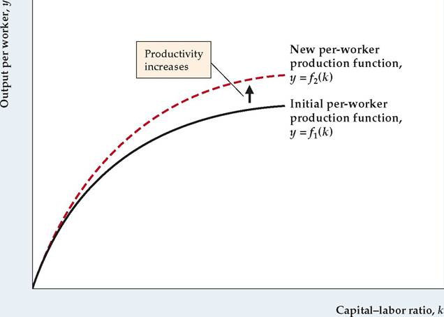
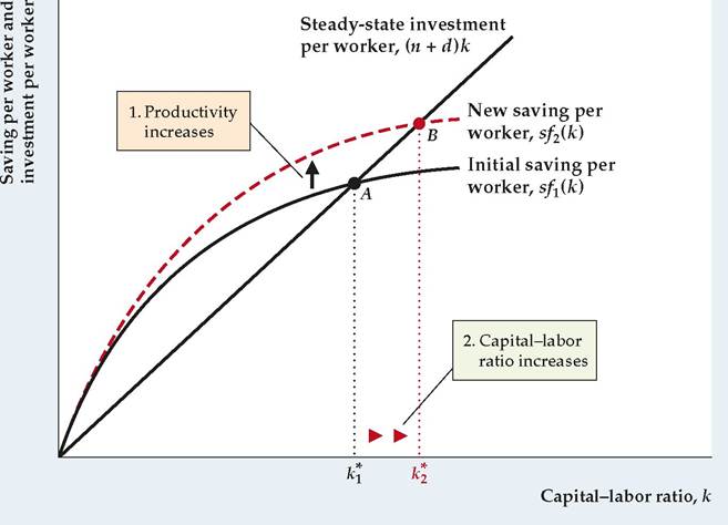
The effects of a productivity improvement—the result of, say, a new technology— are shown in Figures 6.8 and 6.9. An improvement in productivity corresponds to an upward shift in the per-worker production function because, at any prevailing capital-labor ratio, each worker can produce more output. Figure 6.8 shows a shift from the original production function, y = f1 (k), to a "new, improved" production function, y = f 2 (k). The productivity improvement corresponds to a beneficial supply shock, as explained in Chapter 3.
Figure 6.9 shows the effects of this productivity improvement in the Solow model. As before, the initial steady state is determined by the intersection of the saving curve and the steady-state investment line at point A; the corresponding steady-state capital-labor ratio is k *. The productivity improvement raises output per worker for any level of the capital-labor ratio. As saving per worker is a constant fraction, s, of output per worker, saving per worker also rises at any capital-labor ratio. Graphically, the saving curve shifts upward from sf1 (k) to sf2 (k), now intersecting the steady-state investment line at point B. The new steady-state capital-labor ratio is k 2, which is higher than the original steady-state capital-labor ratio, k *.
FIGURE 6.8
An improvement in productivity
An improvement in productivity shifts the per-worker production function upward from the initial production function, y = f1 (k), to the new production function, y = f2 (k). After the productivity improvement, more output per worker, y, can be produced at any capital-labor ratio, k.
Overall, a productivity improvement raises steady-state output and consumption per worker in two ways. First, it directly increases the amount that can be produced at any capital-labor ratio. Second, as Fig. 6.9 shows, by raising the supply of saving, a productivity improvement causes the long-run capital-labor ratio to rise. Thus a productivity improvement has a doubly beneficial impact on the standard of living.
Like a one-time increase in the saving rate or decrease in the population growth rate, a one-time productivity improvement shifts the economy only from one steady state to a higher one. When the economy reaches the new steady state, consumption per worker once again becomes constant. Is there some way to keep consumption per worker growing indefinitely?
In reality, there are limits to how high the saving rate can rise (it certainly can't exceed 100%!) or how low the population growth rate can fall. Thus higher saving rates or slower population growth aren't likely sources of continually higher living standards. However, since the Industrial Revolution, if not before, people have shown remarkable ingenuity in becoming more and more productive. In the very long run, according to the Solow model, only these continuing increases in productivity hold the promise of perpetually better living standards. Thus we conclude that, in the long run, the rate of productivity improvement is the dominant factor determining how quickly living standards rise.
Economic Models, Endogenous Variables, and Exogenous Variables
The Solow model provides a useful framework for analyzing growth and illustrates several features of many different types of economic models—equilibrium conditions, endogenous variables, and exogenous variables.
FIGURE 6.9
The effect of a productivity improvement on the steady-state capital-labor ratio
A productivity improvement shifts the production function upward from f1 (k) to f 2 (k), raising output per worker for any capital-labor ratio. Because saving is proportional to output, saving per worker also rises, from sf1 (k) to sf 2 (k). The point where saving per worker equals steady-state investment per worker shifts from point A to point B, and the corresponding steady-state capital-labor ratio rises from k * to k *. Thus a productivity improvement raises the steady-state capital-labor ratio.
Equilibrium Conditions. Economists solve models by finding a point of equilibrium. In the Solow model, the steady-state equilibrium occurs where in Fig. 6.5 the two lines cross, depicting the level of steady-state capital per worker at which steady-state investment per worker equals saving per worker. The graph shows the one point that satisfies Eq. (6.11), so we call that equation the equilibrium condition. Much of theoretical economic analysis involves developing a model that explains an economic situation and finding the equilibrium condition or conditions.
Exogenous Versus Endogenous Variables. No economic model can develop an equilibrium condition for every possible variable. Instead, some variables are taken as given, and the values of other variables are determined by the equilibrium of the model. A variable that is taken as given is called an exogenous variable. A variable that is determined by the equilibrium in the model is called an endogenous variable. For example, in the Solow model, we take the values of the variables n, s, and d as given. The model does not determine these variables, so they are exogenous variables. However, given the values of n, s, and d and knowledge of the production function, f, we can determine the values of variables k, y, and c, so those variables are endogenous. To see this, note that Fig. 6.5 and thus Eq. (6.11) determine the value of n. Then we can use Eq. (6.5) to determine y and use Eq. (6.8) to determine c.
When economists analyze an economic model, the most common type of question they can answer is: How does a change in an exogenous variable affect all the endogenous variables? For example, the analysis shown in Fig. 6.6 shows how a higher saving rate (an exogenous variable) affects the steady-state value of k (an endogenous variable). Then Eqs. (6.5) and (6.8) can be used to show how the steady-state values of y and c change because of the higher saving rate. Similarly, Fig. 6.7 shows the impact of a higher population growth rate. In a similar vein, because we took the production function, f, as given, we can analyze the impact of a change in productivity, as in Fig. 6.9, on the endogenous variables.
Some types of questions posed in analyses of economic models are not well posed or meaningful. For example, it is meaningless to ask how an endogenous variable affects an exogenous variable. So, suppose someone were to ask you: How does a higher steady-state capital stock affect the rate of population growth? Your answer would be: I cannot answer the question with the Solow model because the rate of population growth is an exogenous variable in the model. To answer that question, you would need a different model in which population growth is endogenous rather than exogenous. Developing a model with a good choice of exogenous and endogenous variables is one of the most important jobs of research economists.
Another meaningless question is to ask how one endogenous variable affects another one. You cannot answer the question: How does a change in steady-state consumption per person, c, affect steady-state capital per person, k, in the Solow model? Because both c and k and endogenous, you should first examine what change in an exogenous variable caused the change in c. The ultimate cause of a change in c must be some change in an exogenous variable or in the production function, which is also taken as given.
In subsequent models in the textbook, identifying which variables are exogenous and which are endogenous, along with finding the equilibrium conditions, will be a major part of the analysis.
Application
The Growth of China
China has experienced soaring growth rates in recent years. Because of its size (population of 1.4 billion), China could become the next great world economic power. Although it has grown rapidly in the past few decades, China started from such a low level of GDP per capita that the country has a long way to go before its GDP per capita catches up to GDP per capita in advanced economies.
Table 6.4 shows that China's GDP per capita compares poorly with other countries. Moreover, real GDP per capita in China was actually lower in 1950 than it had been 80 years earlier in 1870. As recently as 2000, China's real GDP per
TABLE 6.4
Economic Growth in China, Japan, and the United States
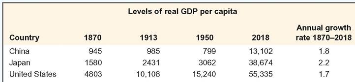
Note: Figures are in U.S. dollars at 2011 prices, adjusted for differences in the purchasing power of the various national currencies.
Source: Data from The Maddison-Project, www.ggdc.net/maddison/maddison-project/home.htm, 2020 version.
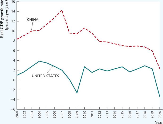
FIGURE 6.10
Real GDP growth in China and the United States, 2001-2020
The chart shows annual values for real GDP growth for both China and the United States for the period 2001-2020. Source: Data from International Monetary Fund, World Economic Outlook, available at www.imf.org/en/Publications/ WEO/weo-database/2021/October.
capita was only about 13% of Japan's, even though China's real GDP per capita was 65% of Japan's real GDP per capita in 1870.
In recent years, real GDP growth in China has been quite rapid. Figure 6.10 shows the growth rate of GDP in China compared with that in the United States. Over the period 2001-2020, China's GDP growth rate averaged 8.7% per year, whereas the U.S. GDP growth rate averaged just 1.7% per year. Analysts have attributed the rapid growth rate in China to a tremendous increase in capital investment, fast productivity growth that has arisen in part from the transition from a centrally planned economy to a market economy, and increased trade with other countries.
Will China be able to maintain its extremely high growth rate of GDP? The experience of many other countries suggests that periods of rapid economic growth by developing economies are often followed by substantial slowdowns in economic growth.24 In the early stages of economic development, developing countries like China often grow much faster than advanced economies like the United States. This rapid growth arises as developing economies make more effective use of underemployed resources, such as labor, take advantage of more advanced technology developed elsewhere, or make important economic transitions such as from a centrally planned economy to a market economy with protection of property rights. But as economic growth progresses in a developing economy, underemployed resources are not as plentiful, technology has moved closer to the level in advanced economies, and the benefits of moving to an improved economic system have been largely exhausted. At that point, economic growth inevitably slows
down. Looking forward, we cannot say when China's growth will slow down, nor by how much. However, we can say that if, starting from the levels of GDP per capita in 2018, China somehow managed to increase its GDP per capita by 10% per year while GDP per capita in the United States grows by only 1% per year, it would take about 17 years for China's GDP per capita to catch up with that in the United States. But if China's growth rate of GDP per capita were to average only 5% per year (still a very impressive growth rate) while U.S. GDP per capita grows 1% per year, it would take 37 years for GDP per capita in China to catch up to the level in the United States.
24See Barry Eichengreen, Donghyun Park, and Kwanho Shin, “When Fast Growing Economies Slow Down: International Evidence and Implications for China,” Asian Economic Papers, Winter/Spring 2012, pp. 42-87.
6.3