Models, Variables, and Functions

Before I introduce the intertemporal approach, it is worth briefly reviewing the nature of mathematical models in macroeconomics.

Scientific models can be thought of as imaginary, simplified versions of the aspect of the world being studied.

Macroeconomic models are thus simplified representations of economies, which allow us to analyze their salient characteristics. Although there is no inherent reason why a model must be mathematical, mathematical models ensure internal consistency in our reasoning about actual economies. They also allow us to handle a greater degree of complexity than nonmathematical models and also to assess the quantitative significance of various factors. It is for these reasons that macroeconomic models are expressed in mathematical form.

Mathematical macroeconomic models consist of variables, functions, and parameters. They are meant to describe the outcome of the behavior and the interactions of economic agents, such as households, firms, the government, and government agencies (such as central banks).

The behavioral rules of economic agents can be postulated directly or derived by making assumptions about the preferences and constraints faced by these agents and then using the main postulates of rational choice on which microeconomics is based. Methods of mathematical optimization allow us to model the behavior of agents that maximize their objective functions under appropriate constraints.

Mathematical economic models typically take the form of systems of equations, designed to describe the structure of the economy in question and the behavior of economic agents.

The equations relate variables to one another and are meant to be behavioral relations, accounting identities, or equilibrium conditions. Variables refer to economic magnitudes that can take different values. There is an important distinction between endogenous variables (i.e., variables whose values are determined by the model itself) and exogenous variables, whose values are determined outside the model and are taken as exogenously given.

Another important element of mathematical models is a set of parameters, usually assumed constant and exogenously given. Parameters relate to the objective functions and constraints of economic agents, and they eventually determine the relations among endogenous and exogenous variables in the model.

Equations in mathematical models take the form of mathematical functions, which describe the relation of a particular variable to other variables in the model. Functions can be linear or nonlinear.

Variables and parameters of functions are usually defined in terms of real numbers. Real numbers can be thought of as points on an infinitely long line called the “number line” or “real line,” where the points corresponding to integers are equally spaced. Any real number can be determined by a possibly infinite decimal representation, such as that of 8.632. The real line can be thought of as a part of the complex plane, and complex numbers include real numbers.²

Examples of such intertemporal macroeconomic models follow in the remainder of this chapter.

2.2 General Equilibrium in a One-Period Competitive Model

To gain a better understanding of the intertemporal approach, and its differences from nonintertemporal approaches, we first analyze a one-period competitive macroeconomic model without savings and investment.

In this model, we assume that there is a continuum of identical households with the same capital and labor endowments and the same preferences. Households live only for one (the current) period. We can thus analyze the behavior of the representative household with a one-period horizon. We shall maintain the concept of a representative household throughout this chapter. We also assume a continuum of identical competitive firms, who hire capital and labor from households and produce a homogeneous output. Because all firms are identical and trade at the same factor and output prices in competitive markets, we only analyze the behavior of one of them, the representative firm.

2.2.1 Endowments, Preferences, and the Optimal Behavior of Households

The representative household lives for one period and is characterized by its endowments and its preferences. We assume that the representative household is endowed with one unit of capital and one unit of labor. Its endowment of capital and labor can be rented to private firms at a competitive rental price of capital r and a competitive real wage w, respectively. Capital and labor are used by competitive firms in the production of a single good y, which has the same characteristics as the capital endowment of the household. The household can use the income from the rental of its capital and labor endowments for consumption, and it can also consume its capital endowment at the end of the period.

Denoting the stock of capital rented to private firms by k, the volume of labor services rented out by l, and the volume of consumption by c, the resource constraints of the representative household are given by

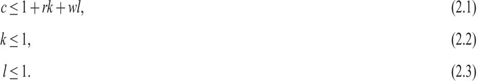
(2.1) indicates that consumption cannot exceed the sum of the income and the capital endowment of the household.

We assume that the preferences of the representative household are described by a continuous, twice differentiable, concave utility function u, which depends on the volume of consumption c of the single good:

The utility function (2.4) satisfies

Thus, the marginal utility of consumption is assumed positive but diminishing. The assumption of a strictly positive marginal utility at all levels of consumption implies that the preferences of the representative household are characterized by nonsatiation. Hence, the representative household always prefers more to less consumption.

The Lagrange function for the problem of the maximization of (2.4), subject to the constraints (2.1), (2.2), and (2.3), can be written as

where λ₁, λ₂, λ₃ are the Langrange multipliers for the constraints (2.1), (2.2), and (2.3), respectively.⁴

The first-order conditions for a maximum are

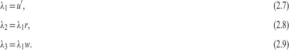
The interpretation of these first-order conditions is straightforward. (2.7) implies that the shadow price of the budget constraint (2.1), λ₁, will be positive, because the marginal utility of consumption is always positive. Hence, the household will consume all its current income plus its capital endowment at the end of the period. The budget constraint (2.1) will be satisfied with equality.

Because λ₁ is positive, (2.8) and (2.9) imply that λ₂ and λ₃ will also be positive for a positive real rental price of capital r and a positive real wage w.

Hence, from the assumption of nonsatiation, embodied in (2.4) and (2.5), the household will rent out its full capital and labor endowment as long as it earns a positive rental price r for capital and a positive real wage w for labor. It will also consume all of its income plus its capital endowment. As a result, the household will choose c to maximize (2.4), subject to the constraints (2.1), (2.2), and (2.3) holding with equality. As a result, the supply of capital and labor to firms and consumption demand will be equal to, respectively,

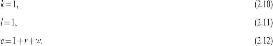
Thus, by maximizing its utility subject to its endowments and its budget constraint, the representative household will commit its full endowments to rental and production; and it will consume all its current income plus the endowment that can be consumed, such as the capital stock.

This completes the discussion of the optimal decisions of the representative household.

Exercise 2.1 Assume that the representative household is endowed with k₀ units of capital and l₀ units of labor. Derive the quantities of capital and labor rented out to private firms, assuming that the household maximizes utility subject to the relevant resource constraints in this case.

2.2.2 The Production Function and the Profit-Maximizing Behavior of Firms

Output is produced by competitive firms, who rent the factors of production (such as capital and labor services) from households through competitive factor markets. All firms have access to the same technology and factor markets, and they produce a homogeneous output y, through the following neoclassical production function:

A is an exogenous technological parameter denoting total factor productivity, and F is a continuous, twice differentiable, quasi-concave function.

From the assumptions we have made, the first and second derivatives of the production function satisfy

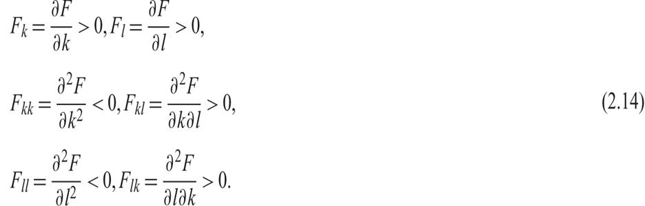
The marginal product of both factors of production is positive but diminishing. In addition, the marginal product of each factor is a positive function of the employment of the other factor.

Constant returns to scale imply that if all factors of production are multiplied by any nonnegative real number—say, μ—the scale of production is also multiplied by μ. Thus, (2.13) also satisfies

for any μ ≥ 0.

Because of the assumption of constant returns to scale, we can multiply all factors by 1/l, and the production function can be written as

where ŷ = y/l is output per worker, and = k/l is capital per worker.

Because of the assumptions about the original production function, the per-worker production function f satisfies the following properties:

Thus, the marginal, and average, product of capital per worker is positive and declining.

Firms are assumed to maximize profits 𝒫. Hence, they choose capital and labor to maximize

From the first-order conditions for a maximum, we have

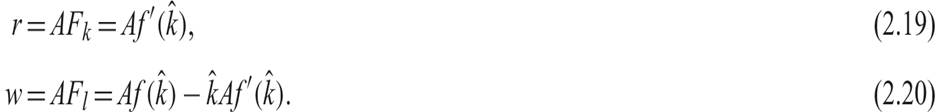
Firms will employ capital and labor up to the point where (i) the marginal product of capital is equal to the rental price of capital r and (ii) the marginal product of labor is equal to the real wage w.

Note that because of the assumption of constant returns to scale, factor payments are equal to total output, and firms make zero profits. From (2.19) and (2.20), it follows that

Thus, because of constant returns to scale, the labor and capital income of households add up to total output.

Because firms operate in competitive markets, they all face the same factor prices. Because they are also assumed to have access to the same technology, they will all choose the same quantities of capital and labor. Thus, we can confine our analysis to the problem of the representative firm. To derive explicit solutions for factor demands and output supply by the representative firm, we have to make explicit assumptions about the production function.

2.2.3 The Cobb-Douglas Production Function

For analytical simplicity, we confine our analysis to the Cobb-Douglas production function of the form⁵

where 0 < α < 1 is a fixed parameter denoting the output elasticity of capital, and 1 − α is the output elasticity of labor.

We can easily confirm that the Cobb-Douglas production function (2.22) satisfies all the assumptions we have made about the neoclassical production function in (2.14) and (2.15). The Cobb-Douglas production function (2.22) is a continuous, twice differentiable, quasi-concave homogeneous function, characterized by constant returns to scale. The marginal product of both factors of production is positive but diminishing, and the marginal product of each factor is a positive function of the employment of the other factor.

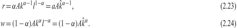
From the marginal productivity conditions (2.19) and (2.20) and the Cobb-Douglas production function (2.22), it follows that

This completes our discussion of the optimal behavior of the representative firm.

2.2.4 General Equilibrium in the One-Period Model

We next turn to the discussion of general equilibrium. Equilibrium employment, output, consumption, real wages, and the real rental price of capital will be determined by (i) the equality of the supply of factors of production by households and the demand for factors of production by firms and (ii) the equality of the demand for and the supply of output.

Because the supply of capital and labor has been shown to be equal to the endowments of the representative household, which have both been assumed to be exogenously given and equal to unity, it follows that capital per worker in production will also be equal to unity. We thus have that

The equilibrium real rental price of capital will be determined in the market for capital, and the equilibrium real wage will be determined in the market for labor, by the equality of the demand and supply for capital and labor.

Substituting (2.25) in (2.23) and (2.24), we find that the equilibrium real rental price of capital and the equilibrium real wage are determined by

where a bar above a variable denotes its equilibrium value.

The equilibrium rental price of capital will be equal to total factor productivity times the share of capital in production, while the equilibrium real wage will be equal to total factor productivity times the share of labor in production. These are the marginal products of capital and labor for a capital-labor ratio equal to one, as implied by our assumptions about the endowments of the representative household.

Note that because the capital and labor endowments have been assumed equal to unity, equilibrium output supply will be equal to total factor productivity and will be given by

Also note that, as shown in (2.21), because of the assumption of constant returns to scale, factor payments to households exhaust output. Firms pay to households the rental price on the capital stock r plus the real wage w. From (2.25), (2.26), and (2.27), one can confirm that, because the endowments are equal to unity, the income of the representative household is equal to

From (2.28), the aggregate income of the representative household is equal to aggregate output.

Equilibrium consumption is then determined by the optimal consumption function (2.12) of the representative household as

From (2.29), households consume all current output plus their initial capital endowment.

This completes the determination of the main macroeconomic variables in the one-period competitive macroeconomic model analyzed in this section. The equilibrium depends on the preferences and the endowments of the representative household and on the technology of production used by the representative firm.

Because of the assumption of nonsatiation, households optimally supply their full endowments of capital and labor to be used for production, and they consume both their current income and their capital endowment.

In equilibrium, the main determinants of real variables are the endowments and preferences of households, the parameters of the technology of production (such as total factor productivity A), and the share of capital α in the case of the Cobb-Douglas production process.

Exercise 2.2 Assume that the representative household is endowed with k₀ units of capital and l₀ units of labor. Derive equilibirum production, consumption, the real interest rate, and the real wage, assuming that households maximize utility subject to the relevant resource constraints, firms maximize profits, and product and factor markets are competitive. Assume a Cobb-Douglas production function of the form of (2.22). Discuss how the equilibrium depends on factor endowments, preferences, and technological parameters.

2.3