Savings and Investment in a Two-Period Competitive Model

The problem of households in the one-period model is relatively simple. Commit your full endowments of capital and labor to production, earn the maximum possible income, and consume all your income plus the endowments that can be consumed, such as the capital stock.

We next turn to a presentation of the simplest possible intertemporal general equilibrium model. This is a two-period model, first analyzed explicitly by Fisher [1930], one of the pioneers of intertemporal macroeconomics. As we shall see, the representative household in a two-period model faces a much wider choice set than in the one-period model.

In a two-period model, the household has to make intertemporal decisions, the most important of which is the savings and investment decision in the first period.

2.3.1 The Representative Household in a Two-Period Model

Assume a representative household, which lives for two periods, say, period 1 (the present) and period 2 (the future). As in the one-period model, the representative household is characterized by its endowments and preferences.

Assume that the representative household is endowed with one unit of capital in period 1 and one unit of labor for each of periods 1 and 2. Also assume that there is no uncertainty and that the household has perfect foresight of developments in period 2.⁶

In period 1, its endowment of capital and labor can be rented to private firms at a competitive rental price of capital r₁ and a competitive real wage w₁. Capital and labor are used by competitive firms in the production of a single good y₁. The household can use the income from the rental of its capital and labor endowments in period 1 for either consumption or investment.

In period 2, the household’s capital stock is equal to its initial capital endowment plus its investment from the first period.

Thus, the main decision of households, apart from the decision to rent out their full endowments of capital and labor to maximize income in each of the two periods, is how much to consume in period 1 relative to period 2. As we shall see, this depends on the future return of investment. Hence, unlike the one-period model, in which the rental price of capital is a pure rent for a fixed endowment, in the two-period intertemporal model, the second-period interest rate acts as an incentive for savings and investment.

The representative household is assumed to maximize the following intertemporal utility function:

where u is a continuous, twice differentiable, concave per period utility function, which depends on the volume of consumption in the period. It has the same properties as the utility function (2.4). Here, ρ > 0 is the pure rate of time preference, which is a measure of household impatience (i.e., of how much the household prefers current to future utility). Because this is a positive parameter, other things being equal, the household is assumed to be impatient: It prefers current to future utility. The utility function (2.30) is characterized by time separability, as intertemporal utility is the weighted sum of per period utilities.⁷

The utility function (2.30) is maximized subject to the following sequence of budget constraints:

Because households are assumed to be endowed with one unit of initial capital k₁ and one unit of labor l per period, and by the assumption of nonsatiation (i.e., they will supply their full endowments for rental in every period), it follows that k₁ = 1, l₁ = l₂ = 1.

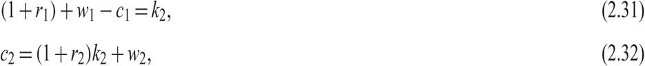
where (2.31) is the budget constraint that applies for period 1. The extent to which the initial capital endowment (assumed equal to unity) plus first-period capital and labor income exceed first-period consumption determines the second-period capital stock k₂. In other words, first-period savings r₁ + w₁ − c₁ are equal to first-period investment k₂ − 1. (2.32) is the budget constraint that applies for period 2. Because this is the last period, the household consumes all of its current income plus the capital stock k₂ carried over from the first period.

The sequence of budget constraints (2.31) and (2.32) can be combined in a single intertemporal budget constraint by using (2.31) to substitute for the period 2 capital stock in (2.32). Then one can show that the intertemporal budget constraint can be expressed as

which is derived from the combination of the sequence of budget constraints (2.31) and (2.32) and is therefore equivalent to them. It states that the present value of consumption is equal to the sum of the period 1 capital stock and its real rent r₁ plus the present value of labor income. Present values are calculated using the period 2 real interest rate r₂, which is the rate of return on savings and investment. Recall that the period 1 real rental price of capital r₁ is a pure economic rent, in the sense that it is the compensation of a factor of production in fixed supply. Real wages are also pure real rents in this model, as labor supply is inelastic.

The right-hand side of (2.33) can be viewed as the wealth of the representative household, consisting of its initial endowment of capital plus the present value of income from its capital and labor endowments.

The problem of the representative household is then to maximize the intertemporal utility function (2.30), subject to the intertemporal budget constraint (2.33). The Lagrange function for this problem can be written as

where λ is the associated Lagrange multiplier. The economic interpretation of λ is that it is the shadow price, or marginal value of household wealth. As long as λ is positive, the value of a marginal addition to the wealth of the representative household is positive.

From the first-order conditions for a maximum, it follows that

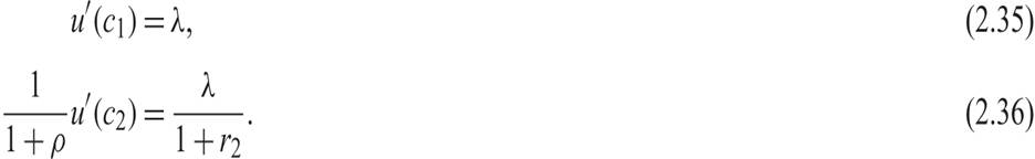
Thus, at the optimum, λ (the marginal value of wealth of the representative household) is equal to the marginal utility of first-period consumption. At the optimum, the household is indifferent between consuming and saving an extra unit of income or wealth. Discounted by the second-period real interest rate, λ is also equal to the marginal utility of second-period consumption. At the optimum, the household has no further incentive to shift consumption from period 1 to period 2, or vice versa.

Dividing (2.36) by (2.35), one gets that at the optimum:

(2.37) is known as the Euler equation for consumption. Its economic interpretation is that the marginal rate of substitution between future and current consumption is equal to the marginal rate of transformation of future consumption into current consumption, or the opportunity cost (price) of future consumption. This opportunity cost is equal to the inverse of 1 plus the real interest rate r₂.

Note that the marginal rate of substitution between current and future consumption depends on the concavity of the per period utility function u, ensuring that indifference curves between current and future consumption will be convex with respect to the origin.

2.3.2 Implications of the Euler Equation for Consumption

The Euler equation for consumption (2.37) can be rewritten as

(2.38) indicates that the ratio of consumption in the two periods depends solely on the relationship between the real interest rate and the pure rate of time preference of the household. The household will smooth its consumption between the two periods by adjusting its savings and investment, according to the relation between the real interest rate and the pure rate of time preference.

If ρ = r₂, then u′(c₁) = u′(c₂) ⇔ c₁ = c₂. If the real interest rate is equal to the pure rate of time preference of the household, then the return on savings is equal to the rate at which the household values the present over the future, and there will be complete consumption smoothing.

If ρ > r₂, then u′(c₁) < u′(c₂) ⇔ c₁ > c₂. If the real interest rate is lower than the pure rate of time preference of the household, then the return on savings is lower than the rate at which the household values the present over the future, savings will be lower, and consumption will be higher in the first period than in the second period.

If ρ < r₂, then u′(c₁) > u′(c₂) ⇔ c₁ < c₂. If the real interest rate is higher than the pure rate of time preference of the household, then the return on savings is higher than the rate at which the household values the present over the future, savings will be higher, and consumption will be lower in the first period than in the second period.

2.3.3 The Case of a Constant Elasticity of Intertemporal Substitution

To further analyze how the consumption path depends on the real interest rate, we will use a special but widely used utility function: the utility function with a constant elasticity of intertemporal substitution (CEIS) of consumption.

where 1/θ is the elasticity of intertemporal substitution of consumption. This utility function is quite general, and versions of it are used extensively throughout this book.⁸

The elasticity of intertemporal substitution of consumption is defined as the percentage change in the ratio of consumption in period 2, relative to consumption in period 1, divided by the percentage change in the marginal rate of substitution between consumption in the two periods, with utility being held constant. It is a measure of the curvature of the intertemporal indifference curves, or the ease with which households can substitute consumption intertemporally. For the utility function (2.39), from the definition above, it can easily be confirmed that this elasticity is constant and is given by 1/θ.

The marginal rate of substitution (MRS) is given by

Hence, the elasticity of intertemporal substitution is given by

In the case where the elasticity of intertemporal substitution is equal to unity, (2.39) is not defined. By using L’Hopital’s rule, one can show that for θ = 1, (2.39) takes the form of logarithmic utility:⁹

Thus, logarithmic utility is a special case of (2.39) when the elasticity of intertemporal substitution of consumption is equal to unity.

For the CEIS utility function (2.39), the Euler equation for consumption can be written as

From (2.41), consumption in the first period satisfies

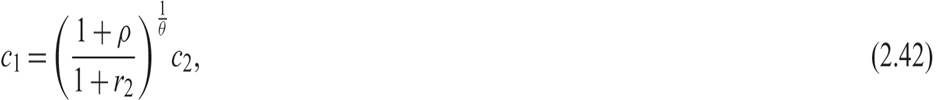
which describes the determination of first-period consumption as a function of the real interest rate and second-period consumption. Combined with the intertemporal budget constraint (2.33), this equation can fully determine the consumption path as a function of the path of real interest rates and real wages.

From (2.42) and the intertemporal budget constraint (2.33), consumption in the first period is determined by

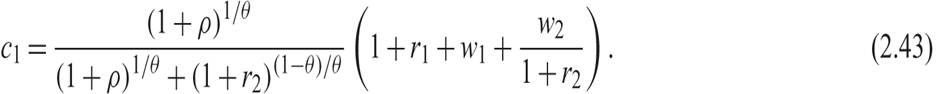
(2.43) is the household consumption function. In the first period, the household consumes a fraction of its total wealth, given by the right-hand side of its intertemporal budget constraint (2.33). The fraction consumed depends on the pure rate of time preference, the second-period real interest rate, and the elasticity of intertemporal substitution 1/θ.

It is straightforward to show that the higher the pure rate of time preference ρ is, the higher will be the fraction of its wealth that the household consumes in the first period. This is logical, as the more impatient the household is, the more willing it will be to bring utility and consumption forward.

It is also straightforward to show that if the elasticity of intertemporal substitution of consumption is higher than unity (i.e., if θ < 1), then the second-period real interest rate r₂ has a negative impact on the fraction of its wealth that the household consumes in the first period. This is because the intertemporal substitution effect is stronger than the income (wealth) effect. Hence, higher real interest rates induce higher savings in this case, as they reduce the relative price of future consumption.

The opposite happens if the elasticity of intertemporal substitution of consumption is lower than unity (i.e., if θ > 1). Then the second-period real interest rate has a positive impact on the fraction of its wealth that the household consumes in the first period. Higher real interest rates induce lower savings, as the intertemporal substitution effect is weaker than the income effect in this case.

In the case where the intertemporal elasticity of substitution is equal to unity (i.e., logarithmic preferences), the fraction of its wealth that the household consumes in the first period is independent of the second-period real interest rate and only depends on the pure rate of time preference. It is given by (1 + ρ)/(2 + ρ). In this case, the intertemporal substitution effect of real interest rates exactly cancels out the income effect.

To fully determine the path of real interest rates and real wages, as well as household wealth, in this two-period model, we have to examine the optimizing behavior of firms and impose the competitive equilibrium conditions.

2.3.4 Firms, Technology, and the Optimal Output Path

As in the one-period model of section 2.2, we assume that output is produced by competitive firms, who rent the factors of production from households through competitive factor markets. All firms have access to the same technology and face the same factor prices. They produce a homogeneous output y, through the neoclassical production function

where t is a discrete time index taking the values 1 and 2, and = k/l. We maintain the assumption that F is characterized by diminishing returns to each factor of production but constant returns to scale, satisfying the properties given in (2.14)–(2.17). Note that A, the exogenous technological parameter denoting total factor productivity, as do the factors of production, capital k and labor l, also depends on the time period. Hence, total factor productivity may differ between periods 1 and 2.

Firms are assumed to maximize profits in both periods. Hence, in every period, they choose capital and labor to maximize

From the first-order conditions for a maximum, we have

Thus, in every period, t = 1, 2, firms will employ capital and labor up to the point where the marginal product of capital is equal to the rental price of capital r, and up to the point where the marginal product of labor is equal to the real wage w. Note that because of the assumption of constant returns to scale, factor payments are equal to total output in every period.

Because firms operate in competitive markets, where they all face the same factor prices, and because they are also assumed to share the same technology, they will all choose the same quantities of capital and labor. Thus, we can again confine our analysis to the problem of the representative firm.

For analytical simplicity, let us employ a Cobb-Douglas production function of the form

where g ≥ 0 is the exogenous rate of technical progress between periods 1 and 2. Hence, g measures the rate of increase in total factor productivity between the two periods.

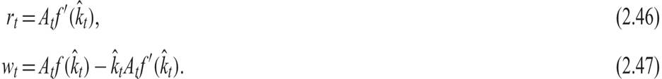
From the marginal productivity conditions (2.46) and (2.47) and the Cobb-Douglas production function (2.48), it follows that

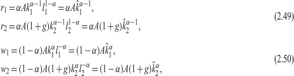
where = k/l.

This completes our discussion of the optimal behavior of the representative firm.

2.3.5 General Equilibrium in the Two-Period Model

We can now turn to the discussion of general equilibrium. Equilibrium employment, output, consumption, investment, real wages, and the real rental price of capital in each of the two periods will be determined by the equality of the supply of factors of production by households and the demand for factors of production by firms, and the supply of output by firms and the demand for output by households.

Because the supply of capital and labor in period 1 has been shown to be equal to the endowments of the representative household, which are both assumed to be equal to unity, it follows that capital per worker in production in period 1 will also be equal to unity:

The real rental price of capital will be determined in the market for capital, and the real wage will be determined in the market for labor, by the equality of the demand and supply for capital and labor. Substituting (2.51) in (2.49) and (2.50), we get that the equilibrium rental price of capital and the real wage in period 1 will be given by

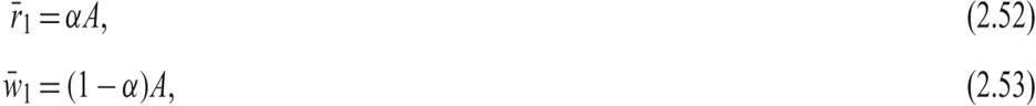
where a bar above a variable again denotes its equilibrium value.

Note that because the capital and labor endowments have been assumed equal to unity in period 1, equilibrium output supply in period 1 is equal to total factor productivity and is given by

Also note that, because of the assumption of constant returns to scale, factor payments to households exhaust output. Firms pay to households the rental price on the capital stock r plus the real wage w. Hence, from (2.52), (2.53), and (2.54), the income of the representative household in period 1 is equal to

The aggregate income of the representative household is thus equal to aggregate output.

Equilibrium consumption in period 1 cannot be determined unless we also analyze equilibrium in period 2, as savings depend on the real interest rate in period 2, which is determined by the marginal productivity of capital in period 2.

In period 2, the endowment of labor continues to be equal to 1. However, the period 2 capital stock may differ from the initial endowment, as a result of savings and investment by the representative household. Thus, although equilibrium factor prices and output in period 1 are determined as a function of the initial endowments of capital and labor and the technology of production in period 1, consumption in period 1 cannot be determined unless we consider the determination of general equilibrium in period 2 as well.

Because the labor endowment in period 2 is equal to unity, it follows that capital per worker will be equal to

Thus, the key is to determine the capital stock in period 2, which will depend on savings and investment in period 1.

The optimal capital stock for period 2 is determined at the point where the marginal rate of substitution between period 2 and period 1 consumption is equal to the marginal rate of transformation, which is equal the inverse of 1 plus the real interest rate of period 2. The condition that determines the capital stock is then (2.43), the Euler equation for consumption. We can rewrite it as

which is the optimality condition that determines the equilibrium capital stock in period 2. Because both c₁ and c₂ depend on the period 2 capital stock through the household budget constraints, and r₂ also depends on the period 2 capital stock through the relevant marginal productivity condition, we need to invoke both the household budget constraints and the marginal productivity condition to determine the equilibrium capital stock.

From the household budget constraints (2.31) and (2.32), after substituting for the equilibrium variables in period 1 from (2.52), (2.53), and (2.54), we have that

From the period 2 marginal productivity condition (2.49) for the real interest rate, we have that

Using (2.58), (2.59), and (2.60) to substitute for c₁, c₂, and r₂ in the optimality condition (2.57), the equilibrium capital stock in period 2 is determined by

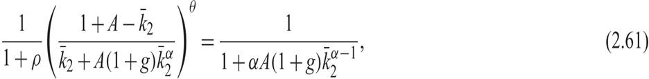
where is the equilibrium capital stock that satisfies equation (2.61). This is a highly nonlinear equation, which cannot be solved analytically. Its interpretation is nonetheless straightforward, and the determination of the equilibrium capital stock can be analyzed with the help of a simple diagram, as in figure 2.1.

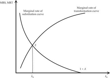
Figure 2.1 Equilibrium capital accumulation in a two-period economy.

The downward-sloping curve in figure 2.1 depicts the left-hand side of (2.61), which is the marginal rate of substitution between period 2 and period 1 consumption. This is a negative function of the second-period capital stock, because as consumers reduce period 1 consumption to increase investment, the marginal utility of first-period consumption rises relative to the marginal utility of period 2 consumption, and hence the marginal rate of substitution falls.

The upward-sloping curve depicts the right-hand side of (2.61), which is the marginal rate of transformation between consumption in periods 2 and 1, again as a function of the second-period capital stock. As investment in the second-period capital stock increases, the real interest rate in period 2 falls, because of the diminishing marginal productivity of capital; hence the marginal rate of transformation between consumption in periods 2 and 1 increases.

The equilibrium capital stock is determined at the intersection of the two curves, where the marginal rate of substitution is equal to the marginal rate of transformation.

If the period 2 capital stock is higher than the equilibrium capital stock, the real interest rate would be lower, and households would immediately reduce savings and investment, reducing the capital stock to its equilibrium value. If the capital stock is lower than the equilibrium capital stock, the real interest rate would be higher, and households would immediately increase savings and investment, increasing the capital stock to its equilibrium value.

To put it differently, the second-period equilibrium capital stock is the stock for which the second-period real interest rate induces households to provide sufficient savings and investment in the first period, so that this capital stock will be attained in the second period.

Note that from (2.61), the optimal second-period capital stock depends on preference parameters, such as the pure rate of time preference ρ and the elasticity of intertemporal substitution of consumption 1/θ, as well as technological parameters, such as A, g, and α. Obviously, it depends on initial endowments as well, which have been normalized to unity.

Having determined the optimal second-period capital stock from (2.61), the rest of the equilibrium variables follow from the household budget constraints (2.58) and (2.59), and the marginal productivity conditions (2.49) and (2.50) for period 2. We thus have that

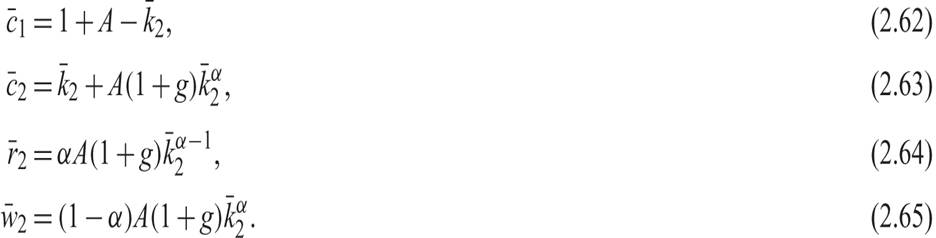
All these variables are determined as functions of the preference, technological, and endowment parameters that determine the second-period capital stock.

Exercise 2.3 Assume that the representative household is endowed with k₀ units of capital and l₀ units of labor and lives for two periods. Derive equilibirum production, consumption, the real interest rate, and the real wage for each period, assuming that households maximize utility subject to the relevant resource constraints, firms maximize profits, and product and factor markets are competitive. Assume a CEIS intertemporal utility function of the form (2.30) and (2.39), and a Cobb-Douglas production function of the form (2.22). Discuss how the equilibrium depends on factor endowments, preferences, and technological parameters.

2.3.6 Diagrammatic Exposition of the Intertemporal Equilibrium

The full intertemporal equilibrium in our two-period model can be analyzed through the use of a simple diagram, as shown in figure 2.2.

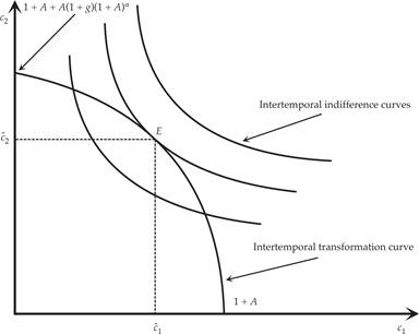
Figure 2.2 Intertemporal equilibrium in a two-period economy.

The preferences of the representative household are depicted by the indifference curves between consumption in period 1 and consumption in period 2. The slope of these intertemporal indifference curves is the marginal rate of substitution between consumption in the two periods.

With a CEIS utility function, as we have assumed, intertemporal household utility is given by

The slope of the indifference curves can be found by totally differentiating the intertemporal utility function (2.66) with respect to c₁ and c₂ and setting the total differential to zero, so that utility remains constant:

From (2.67), it follows that the slope of the indifference curve is given by

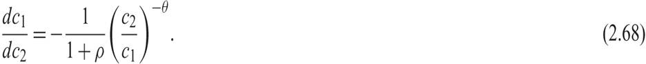
Thus, the slope of indifference curves is equal to the marginal rate of substitution between consumption in the two periods. It is negative and decreasing in the ratio c₁/c₂.

The budget constraint of the representative household is depicted as the intertemporal transformation curve, which shows the maximum consumption that can be attained in one period, subject to a given level of consumption in the other period. The intertemporal transformation curve is essentially the budget constraint of the representative household and depends on endowments and technological possibilities.

Note that if the household maximizes first-period consumption by consuming its capital endowment and all its period 1 income in the first period (i.e., by consuming 1 + A in the first period), then second-period capital and consumption are equal to zero, as there is no capital and no production in the second period. If first-period consumption is equal to zero, then the second-period capital stock is maximized at 1 + A, and second-period consumption is maximized at 1 + A + A(1 + g)(1 + A)^α. The intertemporal transformation curve shows all other feasible combinations in between these two extremes.

The slope of the intertemporal transformation curve can be found by totally differentiating the intertemporal budget constraint (2.33) and setting the total differential to zero:

This is a negative and decreasing function of the capital stock in period 2 (i.e., a negative but increasing function of the ratio c₁/c₂). Hence, the transformation curve is concave to the origin.

Equilibrium is at point E in Figure 2.2, where the transformation curve is tangential to the highest possible indifference curve. This point is the only intertemporal equilibrium for this model, and it is the only point where the Euler equation for consumption (2.57) is satisfied.

Because of the assumption of nonsatiation, the representative household will always choose points on the intertemporal transformation curve. For any point other than E, the household can increase its intertemporal utility by changing its consumption pattern. The only point where the household has no incentive to change its consumption pattern is point E.

2.3.7 Implications for Growth and Business Cycle Theory

The two-period model of savings and investment that we have examined in this section can be seen as the basis of most optimizing one-sector models of economic growth and of competitive models of aggregate fluctuations.

The representative household model of economic growth, one of the workhorses of growth theory, is nothing more than an extension of the two-period model to economies that last for an infinite number of periods. In fact, this extension was accomplished by Ramsey [1928], even before the publication of the two-period model by Fisher [1930].

The Ramsey infinite horizon representative household model of optimal growth is analyzed in chapter 4. Models of overlapping generations (such as the Diamond [1965] and the Blanchard [1985] and Weil [1989] models, which are analyzed in chapter 5) are also based on the two-period intertemporal model of Fisher [1930]. Essentially, they are an extension of the representative household model to economies in which households have different birth dates. However, as we shall see, overlapping generations models do not share the optimality properties of the two-period representative household model or the infinite horizon Ramsey model with perfect markets. The reason is that in the overlapping generations model without intergenerational links, current generations do not take the welfare of future generations into account, and hence savings are lower that what would be socially optimal.

As we shall see in chapters 4–9, which rely on versions of either representative household or overlapping generations models, the invididual household optimality conditions of the two-period model, such as the Euler equation for consumption, recur again and again in these infinite horizon growth models. Hence, their basic properties are related to those of the two-period model, although, obviously, these multiperiod models also have richer and more diverse predictions and implications. However, to the extent that there is no intergenerational altruism, overlapping generations models imply suboptimally low savings.

The two-period representative household model forms the basis of competitive equilibrium theories of business cycles, in the form of the stochastic growth model presented in chapter 13. However, in addition to going beyond the two-period model, this requires introducing the consumption-leisure choice and uncertainty in the form of stochastic real disturbances.

2.4