Consumption and Labor Supply in a One-Period Competitive Model

Up to now we have assumed that the household provides a unit of labor inelastically. Yet in many contexts, it is appropriate to treat employment as a choice variable for households, much like consumption.

As before, we start our analysis with a one-period model, in which households choose both consumption and labor supply. This helps contrast the resulting equilibrium with the intertemporal equilibrium in models with more than one period.

2.4.1 The Optimal Choice of Consumption and Labor Supply

Assume an economy in which the representative household lives for one period and is endowed with one unit of time. For analytical simplicity, we concentrate on the case in which labor is the only factor of production and there is no capital.

Time can be used for leisure activities z, which yield utility to the household, or rented out as labor l to private firms at a competitive wage rate w, and is used in the production of the single good. Denoting the volume of consumption by c, the budget constraints of the representative household are given by

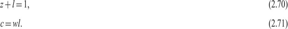
Assume that the preferences of the representative household are described by a continuous, twice differentiable, quasi-concave utility function u, whose arguments are the volume of consumption and the amount of leisure time:

From the quasi-concavity of the utility function, it follows that

From the assumption of nonsatiation, the household will use all its time, either as leisure z or as labor services l.

subject to

The Lagrange function for this problem can be written as

where λ is the Langrange multiplier for the budget constraint (2.75). From the first-order conditions for a maximum, it follows that

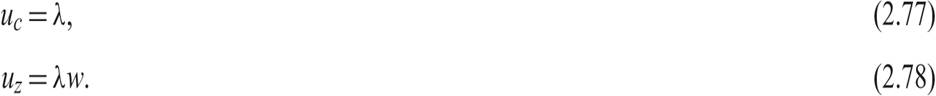
The interpretation of these two first-order conditions is straightforward. At the optimum, the marginal utility of consumption is equal to the marginal valuation of income λ, while the marginal utility of leisure is equal to the marginal valuation of income λ times the real wage w. Hence, at the optimum, the household cannot increase its utility by either increasing or decreasing its labor supply at the expense (or in favor) of leisure.

Dividing (2.78) by (2.77), we get the optimality condition that the marginal rate of substitution between consumption and leisure is equal to the real wage, which is the opportunity cost of leisure:

As one can confirm by totally differentiating the utility function (2.74) and keeping the level of utility constant, the ratio of the marginal utilities of leisure and consumption in (2.79) is equal to the marginal rate of substitution between consumption and leisure:

The optimum is shown diagrammatically in figure 2.3.

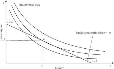
Figure 2.3 Optimal consumption and leisure in a one-period economy.

The optimum is at point E, where the budget constraint is tangential to the highest possible indifference curve. At point E, the marginal rate of substitution between consumption and leisure is equal to the real wage. The household cannot attain a higher level of utility by substituting away from (or toward) more leisure compared to point E.

2.4.2 Income and Substitution Effects on Labor Supply

The effects of changes in the real wage on consumption and labor supply can be analyzed with the help of figure 2.4.

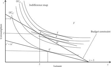
Figure 2.4 Income and substitution effects on labor supply.

In figure 2.4, we assume that originally the economy is at the equilibrium point E. We consider the impact of a reduction of the real wage from w to w′. The budget constraint shifts to one with a smaller slope, and the economy will shift to E′ with lower consumption, because for consumption, the income and the substitution effects are both negative.

Whether labor supply will also fall depends on the relative strength of the income and substitution effects. The income effect points to a reduction in the demand for leisure and an increase in labor supply: The income of the household is now lower, and the household demands less of both consumption and leisure at a lower real income. The substitution effect works in the opposite direction: The opportunity cost of leisure has gone down, and leisure has become relatively less expensive.

In figure 2.4, the substitution effect dominates, and at the new equilibrium E′, the “Marshallian” demand for leisure (which depends on both the income and the substitution effect) has gone up, and labor supply has gone down.

There are at least three ways to isolate the income from the substitution effect of any change in the real wage: The Hicks [1939] method, the Slutsky [1915] method, and the Frisch [1932] method. The Hicks method relies on the assumption of compensating the household to achieve the original level of utility after the change in the real wage. The Slutsky method relies on the assumption of compensating the household to buy the original consumption-leisure bundle after the change in the real wage. The Frisch method relies on the assumption of compensating the household to maintain the same marginal utility of wealth following the change in the real wage. With separable preferences, this is equivalent to assuming that the level of consumption remains unchanged.

The Hicksian substitution effect, which is theoretically the most satisfactory of the three methods, is measured from the movement from E to H, along the original indifference curve in figure 2.4. At point H, the marginal rate of substitution between consumption and leisure is equal to the new lower real wage, but we have assumed that the household has been compensated to achieve the original level of utility. This measures the Hicksian compensated demand for leisure, or equivalently, the compensated supply of labor.

The Slutsky substitution effect is measured from the movement from E to S, along a line that passes through the original consumption-leisure bundle but has the slope of the new budget constraint. At point S, the marginal rate of substitution between consumption and leisure is equal to the new lower real wage, but we have assumed that the household has been compensated so that it can select the original bundle if it wants to.

The movement from point E to point F measures the Frisch demand for leisure (or supply of labor) and is based on the assumption that the household is compensated to achieve the same level of consumption (not utility) as in the original equilibrium, following the decline in the real wage. With time-separable preferences, the same level of consumption implies the same marginal value of wealth.

Marshallian demands are the actual market demands for leisure, following a change in the real wage, whereas Hicksian, Slutskian, and Frischian demands are alternative measures of compensated demands based on different approaches to the isolation of the substitution effect.

2.4.3 The Frisch Elasticity of Labor Supply

To derive explicit solutions for consumption demand and labor supply by the representative household, one has to make explicit assumptions about the utility function.

For reasons of analytical simplicity, we confine our analysis to the following class of additively separable utility functions:

where θ and γ are nonnegative parameters. (2.81) is an additively separable extension of (2.39), the CEIS utility function used in section 2.3.3. It is additively separable in utility from consumption and leisure.

From (2.81), the marginal rate of substitution between consumption and leisure (i.e., the slope of the indifference curves) is given by

From the optimality condition that the marginal rate of substitution between consumption and leisure must be equal to the real wage, it follows that

From (2.83), solving for employment, one can see that the elasticity of labor supply with respect to the real wage, holding consumption constant, is equal to 1/γ.

Hence, the two parameters θ and γ of the utility function (2.81) can be interpreted as the inverse of the elasticity of intertemporal substitution of consumption and the inverse of the Frisch elasticity of labor supply, respectively.

2.4.4 The Production Function and the Optimal Decisions of Firms

Output is produced by competitive firms, who rent labor services from households in competitive labor markets. Firms have access to the same technology and labor markets, and they produce a homogeneous output y through the following linear production function:

where A is an exogenous parameter denoting total factor productivity and possibly a fixed factor of production such as land. Because labor is the only variable factor of production, (2.84) is characterized by constant returns to scale.¹⁰

Firms are competitive and are assumed to maximize profits. Hence, they choose labor to maximize

From the first-order conditions for a maximum, we have

Because firms operate in competitive markets, they all face the same real wage. Because they are also assumed to share the same technology, they will all choose the same quantity of labor. Thus, we can confine our analysis to the problem of the representative firm.

Note that, because of the assumption of constant returns to scale, wage payments to households exhaust output. Firms pay to households the real wage bill wl. Because the real wage w is equal to A, we have

The income of the representative household is thus equal to aggregate output.

2.4.5 General Equilibrium and the Determination of Output and Employment

To determine the employment rate (and through the employment rate, the rest of the endogenous variables), we must consider the equilibrium conditions in product and labor markets. Hence we must combine the optimal decisions of firms with the optimal decisions of households, which will allow us to determine all the endogenous variables.

Using the definition of household income in (2.87) and the budget constraint of the representative household (2.75), we have that consumption is also a function of the employment rate:

which is the equilibrium condition in the product market, ensuring that the consumption decisions of households are compatible with the production decisions of firms. It implies that consumption is equal to total output.

The equilibrium real wage is the one that makes the employment decisions of households, as determined by (2.83), equal to the employment decisions of firms, as determined by (2.86). So these equations imply that

which is the equilibrium condition in the labor market, ensuring that the real wage w is compatible with the employment decisions of both households and firms.

Solving (2.88) and (2.89) simultaneously, we can determine the equilibrium employment rate. The solution for l is given by

where l denotes equilibrium employment.

From (2.90), equilibrium employment will be a positive function of total factor productivity only if θ < 1 (i.e., only if 1/θ, the intertemporal elasticity of substitution of consumption, is greater than unity). Note that if the intertemporal elasticity of substitution of consumption is equal to unity, then equilibrium employment is equal to unity as well.

Equilibrium real wages and equilibrium output and consumption are determined by

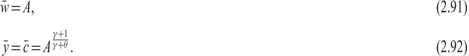
The equilibrium real wage is equal to the exogenous total factor productivity, which is equal to the marginal product of labor for a linear production function.

Equilibrium output and consumption will be positive functions of total factor productivity. If the intertemporal elasticity of substitution of consumption is higher than unity (i.e., θ < 1), then the elasticity of equilibrium aggregate output and consumption with respect to total factor productivity is greater than unity as well, as higher productivity induces higher employment by households and vice versa.

2.5