Fiscal Policy in a Two-Period Competitive Model

Up to this point we have not allowed for the existence of government expenditure and taxes. In this section, we introduce the government and examine how fiscal policy (i.e., government expenditure, taxes, and government debt) affect the economy.

2.7.1 Government Expenditure and Taxes in a One-Period Economy

Assume a one-period economy in which the representative household is endowed with one unit of capital and one unit of labor. Its endowment of capital and labor can be rented to private firms at a competitive rental price of capital r and a competitive real wage w. Capital and labor are used by competitive firms in the production of a single good y. The household can use the income from the rental of its capital and labor endowments for consumption, and it can also consume its capital endowment at the end of the period.

The government can tax the representative household and spend the proceeds on buying the single good y itself. Government expenditure is denoted by c_g. Because this is a one-good economy, government expenditure is on goods that yield utility to the representative household and are perfect substitutes for private consumption. The government pays for government expenditure by imposing a lump sum tax on the representative household, which is denoted by τ.

Because the economy lasts for only one period, the value of taxes must be equal to government expenditure. In this one-period model, the government cannot spend more than its tax revenue, as it would not have the ability to pay, and it will not spend less, as this would imply a waste of resources. Its budget constraint is thus given by

The problem of the representative household is to maximize its utility function u, which depends on the volume of both private and public consumption, subject to its budget constraint and the choice of government expenditure and taxes by the government.

subject to

The last equality in (2.133) is the result of imposing the condition that the household commits to production its full endowments of capital and labor, each of which is equal to unity. As we have already shown, this follows from the assumption of nonsatiation.

From the first-order conditions for a maximum, and after taking account of the optimal behavior of the representative firm (as in the case of subsection 2.2.4) and the government budget constraint (2.131), equilibrium private consumption is given by

where A denotes total factor productivity. In equilibrium, because taxes are equal to government expenditure, government expenditure displaces private consumption one for one, without affecting any other real variables.

Substituting the government budget constraint (2.131) into (2.134), equilibrium aggregate output is given by

This is the same as in the model of subsection 2.2.1 without government expenditure and taxes. One can also show that the equilibrium real rental price of capital and the real wage are given by (2.26), as in the one-period model without a government.

Hence, the only real effect of government expenditure and taxes in this economy would be a one-for-one substitution of public for private consumption, without any other real effects. Aggregate output and employment are the same as in the case where government expenditure and taxes are equal to zero.

The same would apply in this model if taxes were not lump sum but proportional to household income.

where 0 < t_y < 1 is the income tax rate.

Because both the capital and labor endowments are fixed, income taxes would have no effects on the utilization of either capital or labor. The representative household would still commit its full endowments to production. Therefore, income taxes do not imply any distortions in this case. Equilibrium aggregate consumption and output would be the same as in the absence of government expenditure and income taxation. They would be given by (2.135).

Private consumption would be equal to the disposable income of the household plus its capital endowment, but there would be no other real effects from government expenditure and taxes.

2.7.2 Income Taxes and Labor Supply

An income tax would only be distortionary and affect equilibrium employment, output, and consumption, in the case where labor supply is endogenous, as in the model of section 2.4.

Assuming an income tax at a rate t_y in the one-period model of section 2.4, with endogenous labor supply, results in equilibrium employment being equal to

Thus, the presence of income taxation is distortionary in this model, as it reduces the net of tax equilibrium real wage and has a negative effect on labor supply and equilibrium aggregate employment.

The only cases in which income taxation would not have a negative impact on labor supply and aggregate employment are the cases in which either the Frisch elasticity of labor supply 1/γ is equal to zero or the intertemporal elasticity of substitution of consumption 1/θ is equal to zero. In either of these two cases, labor supply is independent of the net of tax real wage.

The elasticity of aggregate employment with respect to the income tax rate is given by

The elasticity of aggregate employment with respect to the income tax rate is not only negative but also increasing in the income tax rate.

In the presence of an income tax and endogenous labor supply, equilibrium aggregate output is given by

It is clear from (2.137) and (2.138) that a positive income tax rate t_y results in lower aggregate employment, output, and consumption, unlike lump sum taxes, which would not affect labor supply.

2.7.3 Government Expenditure, Taxes, and Debt in a Two-Period Economy

We next turn to an analysis of fiscal policy in the two-period model of section 2.3. In this two-period model, labor supply is exogenous, but the savings decision is endogenous. Both the representative household and the government have to make intertemporal decisions. As we have seen, the most important such decision for the household is the savings and investment decision in the first period. For the government, the most important intertemporal decision is whether to finance government expenditure in the first period through taxes or borrowing (government debt).

We assume a government that wishes to finance a stream of primary government expenditure c_g1, c_g2 over two periods. The sequence of government budget constraints is as follows:

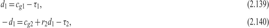
where (2.139) is the period 1 budget balance, which could be a deficit or surplus. To the extent that government expenditure is higher than taxes in the first period, the government runs a budget deficit equal to d₁. This deficit is financed by one-period bonds (i.e., government debt equal to d₁).

(2.139) is the period 2 budget balance. If the government has run a deficit in the first period, then in the second period, it has to run a surplus equal to the deficit of the first period, because the second is the last period and the government has to repay its debt. Thus, tax revenue τ₂ must be sufficient to cover period 2 government expenditure and repayment of the debt. Period 2 government expenditure consists of two elements. First, interest payments on government debt from period 1, plus period 2 primary government expenditure c_g. Primary government expenditure is defined as government expenditure other than interest payments on existing government debt. The period 2 government budget constraint is thus given by equation (2.140).

As in the case of the representative household, the sequence of budget constraints (2.139) and (2.140) can be combined into a single intertemporal budget constraint. Using (2.139) to substitute for government debt in (2.140), after a simple rearrangement, we get

which is the government intertemporal budget constraint. It has an interpretation similar to the intertemporal budget constraint of the representative household. The present value of primary government expenditure in the two periods must be equal to the present value of tax revenue in the two periods. Thus, in an intertemporal setting, the government does not have to balance the government budget in every period, as long as its intertemporal budget constraint of the form of (2.141) is satisfied. It can run a government deficit or surplus in the first period, provided that this is reversed in the second period.

2.7.4 Ricardian Equivalence between Tax and Debt Finance

What are the implications of the government intertemporal budget constraint for the behavior of the economy? Does the method of financing first-period primary expenditure matter?

To address these questions, let us consider the intertemporal budget constraint of the representative household in this case.

Substituting the present value of taxes from the government budget constraint (2.141) into the household intertemporal budget constraint (2.142), we get that the household intertemporal budget constraint is given by

From (2.143) it is clear that only the present value of primary government expenditure affects the intertemporal budget constraint of the representative household. The method of financing primary government expenditure (i.e., tax versus debt finance) has no effect on the household intertemporal budget constraint.

What about the intertemporal utility function of the representative household? In the presence of government expenditure, this is given by

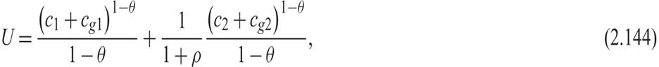
where it is assumed that government expenditure is not wasteful. In fact, government expenditure affects the utility of the representative household in the same way as private consumption. The representative household chooses private consumption to maximize the intertemporal utility function (2.144), subject to the intertemporal budget constraint (2.143).

Note that the method of financing primary government expenditure does not appear either in the utility function of the representative household or in the intertemporal budget constraint. Hence, the only fiscal policy parameters that can affect the optimal decisions of the representative household and the behavior of the economy are related to the path of primary government expenditure. The method of financing the path of government expenditure cannot affect the optimal savings and investment decisions of the representative household. Debt and tax finance are equivalent.

This result, which was first alluded to by Ricardo [1817], is called Ricardian equivalence between debt and tax finance of government expenditure. In effect, the representative household realizes that debt finance is nothing more than a postponement of taxes to the future. Lower current taxes will result in higher future taxes with the same present value. Hence, the only thing that matters for the optimal savings and investment decisions of the representative household is the present value of primary government expenditure that needs to be financed, not the distribution of financing between the two periods. At the end of the two periods, the representative household will need to pay taxes with present value equal to the present value of the stream of primary government expenditure.¹⁵

The first-order conditions for a maximum of (2.144) subject to the intertemporal budget constraint (2.143) are given by

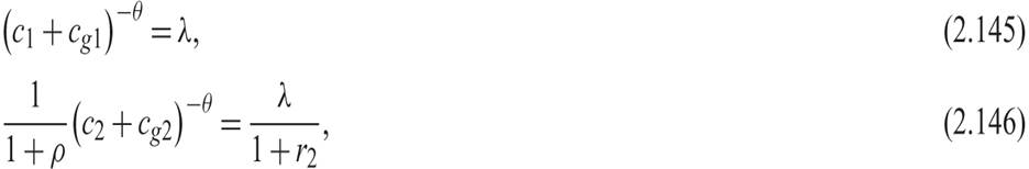
where λ is the Lagrange multiplier measuring the marginal value of wealth.

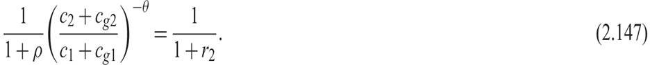
Eliminating λ between equations (2.145) and (2.146), we get the familiar Euler equation for consumption. Consumption is now the sum of private and government consumption:

Taking into account the behavior of the representative firm, which is not affected by government expenditure and taxes, the product market equilibrium conditions in the two periods require that output is equal to the sum of private and public consumption plus investment in every period, which implies that

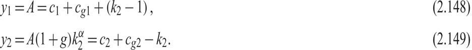
Furthermore, from the marginal productivity condition of the second period, we have that

Using (2.148), (2.149), and (2.150) to substitute for the sum of private and public consumption in the two periods, and the period 2 real interest rate in the Euler equation (2.147), we get that the equilibrium period 2 capital stock will be determined by solving

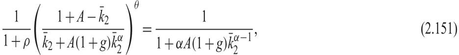
where k₂ denotes the equilibrium capital stock in period 2. Equilibrium investment in period 1 is equal to k₂ − 1, and equilibrium investment in period 2 is equal to −k₂, as the household consumes its capital stock at the end of period 2.

Equation (2.151) is the same as (2.61), which is from the two-period model without government expenditure. Hence, equilibrium investment and the equilibrium period 2 capital stock will not be affected by either government expenditure or the method of financing it. The evolution of real output, aggregate savings, and investment will be the same as in the case where there is no government expenditure, government debt, or taxes.

The only effect of the path of government expenditure in this model is the displacement of an equal amount of private consumption. Since government consumption is assumed to be a perfect substitute for private consumption, neither aggregate savings and investment nor the evolution of real output are affected by the path of government expenditure, debt, or taxes.

This is a striking result. It is due to the assumptions that government expenditure is a perfect substitute for private consumption and that taxes are lump sum (i.e., they do not distort the savings and investment decisions of households). This result would not hold if either government expenditure were an imperfect substitute for private consumption, or if taxes were distortionary and affected the real interest rate faced by households.

2.7.5 Income Taxation and Aggregate Savings and Investment

Although Ricardian equivalence holds for lump sum taxes, an income tax would be distortionary in this model, as it would affect equilibrium savings and investment and second-period output and consumption.

Assuming an income tax rate of t_y, results in the Euler equation for consumption (2.151) amended to

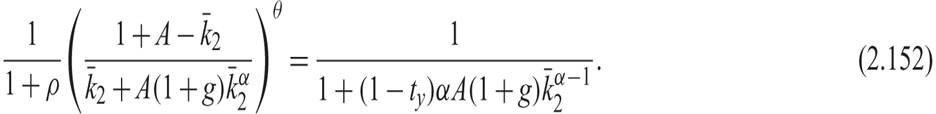
The net of tax real interest rate will be lower at the level of savings and investment without an income tax. Households would thus reduce savings and investment, and the economy will end up with a lower capital stock and output in period 2. Consumption in period 1 will rise relative to consumption in period 2, and savings, investment, and the capital stock in period 2 will be lower.

Thus, with income taxation, the method of financing government expenditure and the level of government expenditure itself will matter for the determination of first-period savings and investment and second-period output and consumption. Ricardian equivalence will no longer hold.

If we allowed for endogenous labor supply as well, income taxation would also distort labor supply decisions, as in the one-period model of subsection 2.7.2.

2.7.6 Implications for Fiscal Policy and Government Debt

The two-period model of fiscal policy analyzed in this section embodies many of the properties of more general intertemporal models of fiscal policy.

Ricardian equivalence is also a property of the infinite horizon, representative household model of economic growth, analyzed in chapter 6. However, in this model, there are full and perfect markets. As we shall see in chapter 6, Ricardian equivalence is not an implication of overlapping generations models of economic growth, in which current generations do not internalize the welfare of future generations. More generally, market distortions (such as the absence of perfect markets for the welfare of future generations) distortionary taxes, or financial distortions lead to a rejection of pure Ricardian equivalence and to potential differences between tax and debt finance of government expenditure. For example, distortionary taxes result in real effects from fiscal policy in all models with endogenous savings or endogenous labor supply.

We return to the impact of distortionary taxation in chapter 6, when we examine capital income taxation and economic growth. In chapter 21, we introduce more general intertemporal models of fiscal policy and investigate the relation between distortionary taxes and the accumulation of government debt.

2.8