The Treatment of Time and the Intertemporal Approach
The two-period intertemporal models examined in this chapter are obviously simplified and restrictive examples. One of the main simplifications is with regard to the treatment of time, which is confined to two time periods only.
Yet the models can be extended in a straightforward manner by allowing for additional time periods.For example, one could assume that time is an integer belonging to any subset of the set of integers ℤ, from minus infinity to plus infinity. Put in mathematical terms, with an infinite number of time periods, we can assume that

or

where ℤ is the full set of integers. Intertemporal analysis could also be confined to any subset of the set of integers ℤ, such as the set of positive natural numbers ℕ, or any finite subset of ℤ or ℕ.
For example, the two-period intertemporal utility function (2.30) of the representative household could be extented to T periods, and take the form

Similarly, the two-period intertemporal budget constraint of the representative household (2.33) could be extended to T periods and takes the form
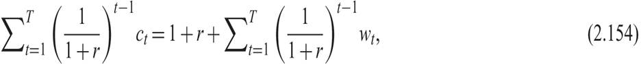
where r is the real interest rate, assumed constant.
When time is expressed in terms of integers, it refers to discrete time periods, such as days, weeks, months, quarters, and years. Such intertemporal analysis is termed discrete time analysis.
Discrete time views values of variables as occurring at distinct, separate points in time, or equivalently, as being unchanged between these points.
Thus, an economic variable that depends on time jumps from one value to another as time moves from one time period to the next. For example, the change of variable x between period t and period t+1 is denoted by

where Δ is called the first difference operator.
This view of time corresponds to a digital clock that displays a fixed reading of 12:00 pm for one minute, then jumps to a new fixed reading of 12:01 pm for the next minute, then to 12:02 pm, and so on. In this framework, each variable of interest is measured once in each time period. The number of measurements between any two time periods is finite. Measurements are typically made at sequential integer values of the discrete variable, time.
Another way to treat time is as a continuous variable. Continuous time analysis views variables as taking a particular value for potentially only an infinitesimally short amount of time. Between any two points in time, there are an infinite number of other points in time. The continuous variable time, denoted by t, ranges over the entire set of real numbers ℝ, or, depending on the context, over some subset of it, such as the nonnegative real numbers. Hence, in continuous time models it is assumed that

We can think of continuous time as the limit of discrete periods of duration Δt, where Δt tends to zero. For example, the change Δ in a variable x between periods t and t + Δt can be written as

Dividing by Δt and letting it tend to zero, we get

A dot above a variable denotes its first derivative with respect to time, when time is a continuous real variable.
In continuous time, the T-period intertemporal utility function (2.153) takes the form

where t is assumed continuous in the interval [0, T]. The integral is the limit of the sum, when the length of the time intervals tend to zero.
Similarly, in continuous time, the T-period intertemporal budget constraint (2.154) takes the form

In subsequent chapters, we use the common convention that t is written as a subscript in an analysis using discrete time and is treated as an argument (in parentheses) in an analysis using continuous time. We will use both ways of defining time. Growth models will be analyzed mostly in continuous time, whereas stochastic models of aggregate fluctuations will be analyzed mostly in discrete time.
The two types of intertemporal analysis are equivalent, but depending on the context, one of the two methods is either analytically or notationally more convenient.
2.9