Money, Prices, and Inflation in a Two-Period Competitive Model

In the models we have presented so far, money has no role. Yet money performs very important functions in an economy. Money is a unit of account, in terms of which market prices are defined and quoted; a means of payments, which reduces transaction costs; and the most liquid store of value.

In this section, we allow for the role of money as a unit of account and a means of payments in a two-period intertemporal model. We assume that transactions can only take place through the intermediation of money (i.e., by paying cash in advance) and that all prices are quoted in terms of money.

In models with money, one can draw the distinction between real variables, defined in terms of physical quantities (such as the ones we have analyzed so far), and nominal variables, defined in money units (such as the stock of money, price level, inflation, nominal output, nominal wages, and nominal interest rates).

2.6.1 The Representative Household and the Demand for Money

We focus on the two-period model without capital, analyzed in section 2.5. The representative household in endowed with one unit of labor for each of periods 1 and 2. It is also endowed with one unit of money m at the beginning of period 1, which it has to return at the end of the period, and one plus an extra μ units of money in period 2, which it again has to return at the end of the period. It is assumed that − 1 < μ < 1.

Money can be thought of as a separate commodity that is a generally accepted unit of account and means of payments. It could be commodity money, in the form of coins, or paper money, in the form of banknotes. It could even be digital money. The stock of money cannot be consumed, and therefore yields no direct utility. For simplicity, we assume that it cannot be carried over from period to period. It can only be used for current economic transactions.

The representative household is assumed to maximize the following intertemporal utility function:

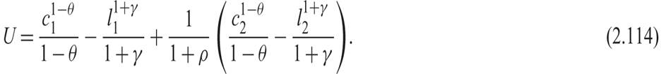
Its intertemporal budget constraint is given by

where p₁ is the money (nominal) price of consumption goods in period 1, p₂ is the money price of consumption goods in period 2, p₁w₁ is the nominal wage in period 1, p₂w₂ is the nominal wage in period 2, and i is the nominal interest rate (i.e., the interest rate expressed in terms of money).

The timing of transactions is assumed to be as follows. In period 1, the household uses its money endowment to buy commodities that cost p₁c₁. At the end of the period, it is paid its money wages p₁w₁l₁ with money. At the end of the period, it also has to repay its money endowment. In period 2, it uses the money it has received for this period, which is one plus the additional money endowment of μ, to buy commodities that cost p₂c₂; at the end of period 2, it is paid its money wages p₂w₂l₂. At the end of period 2, it also has to repay its money endowmnent.¹²

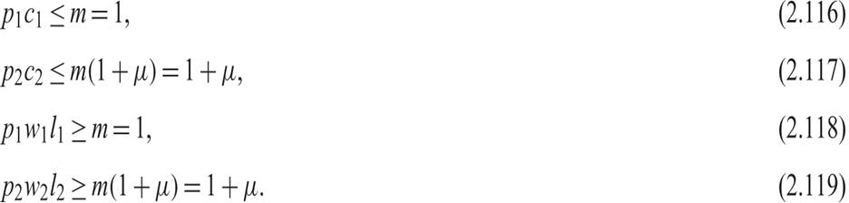
The household has to pay money up front to purchase commodities for consumption. In addition, the household receives money for its labor services in the form of money wages. Hence, there are four additional constraints, usually called cash in advance constraints. These take the form

The Lagrange function for this problem is given by

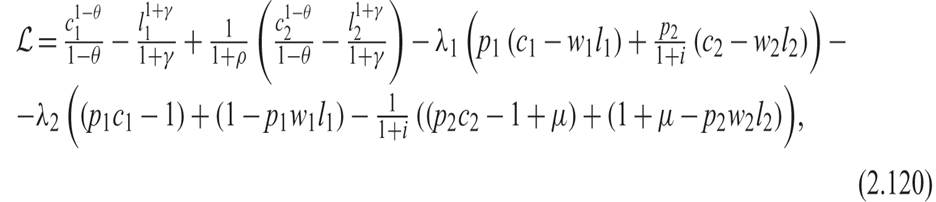
where the Lagrange multiplier λ₁ measures the marginal value of household wealth, and λ₂ measures the marginal value of money.

From the first-order conditions for a maximum, we get that

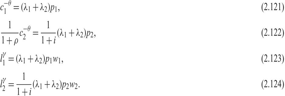
The interpretation of these first-order conditions is straightforward. (2.121) suggests that the marginal utility of period 1 consumption is equal to the marginal value of wealth plus the marginal value of money, multiplied by the period 1 money price of consumption goods. (2.122) suggests that the marginal utility of period 2 consumption is equal to the discounted marginal value of wealth plus the discounted marginal value of money, multiplied by the period 2 money price of consumption goods. (2.123) suggests that the marginal utility of period 1 leisure is equal to the marginal value of wealth plus the marginal value of money, multiplied by the period 1 money price of leisure, which is none other than the period 1 nominal wage. And (2.124) suggests that the marginal utility of period 2 leisure is equal to the discounted marginal value of wealth plus the discounted marginal value of money, multiplied by the period 2 money price of leisure, which is the nominal wage in period 2.

Given the assumption of nonsatiation, the intertemporal budget constraint (2.115) and the cash in advance constraints (2.116)–(2.119) will also be satisfied with equality. As a result, the demand for money in every period will be proportional to household consumption and/or income, whichever is higher. Thus, the demand for money in this model is determined by a simple version of the quantity theory of money.¹³

2.6.2 The Classical Dichotomy and the Neutrality of Money

Eliminating λ₁ + λ₂ between (2.121) and (2.122) gives us the Euler equation for consumption:

where π = (p₂/p₁) − 1 is the rate of change of money prices (i.e., the inflation rate) between periods 2 and 1.

As first defined by Fisher [1896], the relationship between the real interest rate r and the nominal interest rate i is given by

This equation is the exact form of the so-called Fisher equation, which states that the real interest rate is defined by the ratio of one plus the nominal interest rate and one plus expected inflation.¹⁴

Note that for a low r and a low inflation rate π, we have

Hence, (2.126) implies that

(2.127) is the approximate form of the Fisher equation, which is often used in place of (2.126) and is relatively accurate only when inflation rates are low.

From (2.125) and (2.126), the Euler equation for consumption in the two-period model with money has the same form as the Euler equation for consumption in the two-period models without money. The marginal rate of substitution between period 2 and period 1 consumption is equal to the inverse of one plus the real interest rate.

Eliminating λ₁ + λ₂ between (2.121) and (2.123) and between (2.122) and (2.124) gives us the optimality conditions for the choice between consumption and leisure in each period. These are the same as equations (2.101) and (2.102) in the two-period model without money. The marginal rate of substitution between consumption and leisure is equal to the real wage in each period.

Finally, dividing the intertemporal budget constraint of the representative household (2.115) by p₁ and using the definition of the real interest rate from (2.125), we get back to (2.94), the intertemporal budget constraint of the representative household in the model without money.

Hence, making the same assumptions about the behavior of firms as in the model without money, the evolution of real variables in the monetary model of this section and the nonmonetary model of section 2.5 will be exactly the same. The evolution of real variables will be determined as in equations (2.109)–(2.113) in section 2.5.4.

The existence of money and monetary growth does not affect the optimal decision rules of either households or firms concerning the determination of real variables. Money matters for nominal but not for real variables. This property is called the classical dichotomy and implies the neutrality of money. It is a property characterizing both static and intertemporal general equilibrium models with optimizing households and firms.

From the cash in advance constraints (2.116) and (2.117) and the determination of equilibrium real consumption and output from (2.113), equilibrium nominal prices will be determined by

Thus, equilibrium nominal prices are equal to the ratio of the money stock to equilibrium real output and consumption.

Equilibrium inflation is determined by

From (2.129), we have that if the intertemporal elasticity of substitution of consumption is equal to unity, then the equilibrium inflation rate is equal to the difference between the rate of growth of the money supply μ and the aggregate growth rate g. Otherwise, equilibrium inflation is equal to the difference between the rate of growth of the money supply and a multiple (γ + 1)/(γ + θ) of the growth rate.

Equilibrium nominal wages will be equal to the product of equilibrium prices from (2.128) and equilibrium real wages from (2.112).

From (2.127), (2.129), and (2.110), the equilibrium nominal interest rate is equal to

From (2.130), if the intertemporal elasticity of substitution of consumption is equal to unity, then the equilibrium nominal interest rate is equal to pure rate of time preference plus the rate of growth of the money supply.

2.6.3 The Two-Period Competitive Model and Classical Monetary Theory

The two-period model with money analyzed in this section embodies most of the basic postulates of classical monetary theory. This model implies the quantity theory of money in the form of the cash in advance constraints (2.116)–(2.119). Households demand money to purchase goods, and they accept money in payment for their labor services.

The model also implies the classical dichotomy, whereby real factors determine real variables (such as output, employment, real wages, and the real interest rate), and monetary factors determine only nominal and monetary variables (such as the price level and nominal wages, and interest rates) as well as inflation. Through the classsical dichotomy, the model thus implies the neutrality of money.

We shall examine extensions of the two-period monetary model to growth models where households have an infinite horizon in chapter 7. In chapter 12, we also examine stochastic general equilibrium models of money demand, introducing uncertainty. In chapters 14–17, we examine the role of money in new classical and new Keynesian DSGE models of aggregate fluctuations. Because of the assumption of nominal price and wage sluggishness, new Keynesian models do not imply classical neutrality in the short run, and they imply than even nominal disturbances can generate fluctuations in real variables, such as output and employment. In chapters 19 and 20, we take an integrated and detailed look at the role of monetary policy in the context of models with nominal rigidities and financial frictions.

The main predictions of extended intertemporal models with full and competitive markets are closely related to the properties of the two-period intertemporal model with money, such as the model examined in this section. The new Keynesian models discussed in chapters 16, 17, 19, and 20 are based on the sluggish adjustment of prices and nominal wages and imply short-run deviations from the neutrality of money and a significant role for monetary policy as a stabilization policy instrument. The intertemporal models with financial frictions discussed in chapters 19 and 20 also imply a modified role for monetary policy, but through channels other than the adjustment of nominal interest rates.

2.7