Problems of Economic Dynamics

7.1.1. Economic hard times...

I went to university in the fateful 1930, and during the four-year course I watched the almost complete collapse of the American economy. I also had occasion, at that time, to hear my Professor of Banking, who was also the Vice-President of the New York Federal Reserve, admitting during a lecture that he did not know why the President had ordered the closure of all the banks the day before.

Thus R. M. Goodwin (‘Economia matematica: Una visione personale’, 1988, p. 157) explained his simultaneous conversion to Marxism and economics. This was not an isolated case; similar conversions flooded in during those years.

The entire period from the beginning of the First World War to the end of the Second was marked by crisis; a crisis which affected every sphere of bourgeois life, from the economic to the social and from the political to the cultural. The outbreak of the First World War had sown doubts about the rationality of the international capitalist system. But the most lucid minds had immediately understood the deep reasons for the conflict, and could not avoid acknowledging the truth in the arguments of those Marxist thinkers who had preached the dangers of imperialism and prophesized the great war. Then, as soon as the First World War had ended, the conditions were laid down for the Second, as Keynes and a few other enlightened thinkers immediately understood.

In the meantime, a nation-continent had attempted its escape from cap­italism with the Bolshevik Revolution, an attempt which not even military intervention by the major capitalist powers was able to quell.

And if this were not enough to convince even the most optimistic of the depth of the crisis, they only had to look at the economy: the breakdown of the system of international payments, abandonment of the Gold Standard even by those countries which still supported it, competitive devaluations, harsh protectionism, the contraction in international trade; and then, increasing instability in growth, increasingly bitter crises, rampant unem­ployment, the Wall Street Crash, and the suicides of speculators. It seemed that all the Marxist predictions were turning out to be true, from the falling rate of profit to the increasing immiseration of the proletariat, from the deepening of the interimperialist contradictions to the reawakening, because of the crisis, of the revolutionary consciousness, and from the increase in the concentration of capital to the amplification of the periodic oscillations. Was the final collapse in sight?

Nobody was surprised at the weakening of the intellectual fascination of that economic orthodoxy which preached the allocative efficiency of com­petition and the rationality of economic agents. Nor was it surprising if the laissez-faire ideology could no longer recruit members, while the most enlightened economists began to theorize the necessity of abandoning free trade in order to rescue capitalism.

The economists of this period can be roughly divided into three groups.

In the next three sections of this chapter we will outline the three most important dynamic theories formulated in the years of high theory, those of Keynes, Kalecki, and Schumpeter. In the rest of this section we will consider various themes of economic dynamics to show the main directions of theoretical development from which originated the work of the three masters. Finally, in the next chapter, we will deal with developments in micro­economic and the general-equilibrium theory as well as with the contributions of various heterodox theories.

7.1.2. Money in disequilibrium

Up to now we have emphasized the static character of neoclassical analysis. In this chapter we must contradict ourselves. In fact, some dynamic macro­economic models had already been formulated in the 1890s by a few great neoclassical economists.

The early neoclassical economists, who were all concerned with other matters, rather overlooked monetary problems and adopted the equation of exchanges as the last word in regard to the scientific explanation of the price level. As we have seen in the last chapter, in Fisher’s (simplified) version, the identity

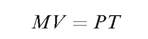
where M is the quantity of money, V is its velocity of circulation, P the level of prices, and T the level of transactions, becomes an explanation of the value of money once V, T, and M have been fixed exogenously. The dif­ficulties and the interesting thing about this theory arise, as Cantillon and Hume had already pointed out, as soon as one wishes to study the process by which a monetary impulse affects the level of prices, that is, as soon as one wishes to tackle the problem of the value of money in dynamic terms. Fisher, Wicksell, and Marshall have made the most interesting attempts to solve this problem. Even though their theories were formulated in the 1890s, it is worth discussing them in this chapter, as they produced their best fruits precisely in the years of the ‘high theory’.

In Fisher’s theory, the variables appearing in the equation of exchanges are set at their normal value, so that the explanation emerging from the equation refers only to the ‘final and permanent effects’ of monetary changes.

Another great influence on the monetary thought of the 1930s, especially in England, was that of Marshall. The Marshallian version of quantity theory is represented by the famous ‘Cambridge equation’. The first official formulation of this theory was made by Marshall in a testimony to the ‘India Committee’ in 1899. As early as 1871, while reformulating Mill’s arguments on money, Marshall had already sketched out his own personal version of the quantity theory in an unpublished paper. For a long time, however, the Cambridge monetary theory remained basically an oral tradition. The key formulations came out rather late, and are to be found in an article by Pigou, ‘The Exchange Value of Legal Tender Money’ (1917), and in Marshall’s Money, Credit and Commerce (1923). The ‘Cambridge equation’ is:

where Y is the real income and h is the ratio in which individuals wish to keep liquid assets. Although h can be interpreted as the inverse of the income velocity of circulation, the original interpretation, which underlines its dependence on the decisions of economic agents, offers quite marked the­oretical advantages.

Another important Marshallian idea in regard to monetary dynamics concerns periodical crises, which Marshall explained as caused by changes in the entrepreneurs’s inflation expectations in connection with credit fluctua­tions. When credit expands excessively and prices rise, entrepreneurs and speculators expect further price rises; therefore they increase their demand for credit and goods. Thus the inflationary expectations are self-fulfilling. As monetary wages are inelastic in the short run, profits increase, investments are encouraged, and inflation is fuelled. In inflationary phases credit expands very fast, which puts the creditors in a risky position and reduces their willingness to offer further credit. At a certain point credit begins to contract and the interest rate rises. A lack of confidence spreads and speculators are forced to sell to repay debts. Thus, prices fall and real wages rise; panic

creates panic, and spreads together with bankruptcies. In the end, production and employment contract. A precise type of monetary policy was derived from this theory, one based on the necessity to stabilize the price level, to control credit, and to establish an indexation of future payment contracts. Rather than Marshall, however, it was his students, especially Pigou and Keynes, who pursued this line of thought. The theory used by Keynes in Tract on Monetary Reform (1923) is inspired by it.

7.1.2. The Stockholm School

An important source of dynamic analysis during the years of high theory was represented by Wicksell’s work. We have already discussed this in the last chapter. Here we will recall the essential elements of Wicksell’s contribution to monetary analysis, just to introduce the theories of his followers. Towards the end of the last century and the beginning of ours, Wicksell undertook a detailed study of the implications of the divergence between natural and bank interest rates and, more importantly, he formulated the nucleus of a theory which aimed to provide the basis for economic policy measures able to guarantee price stability.

In Wicksell’s theory, the ‘natural’ interest rate is the equilibrium price of savings and investments, and, at the same time, the real rate of returns of investments. However, the ability of the banks to create credit is independent from savings, so that the market interest rate, i.e. the one applied to bank credit, can differ from the natural rate. If it is lower, the demand for credit will increase. The supply of credit will adjust, as it is fairly elastic (even if not completely, given the necessity of the banks to maintain reserves). The monetary expansion will fuel the demand for real goods and, with it, increase prices. This is a disequilibrium inflationary process in which Say’s Law does not apply. As long as the difference between the natural and market interest rates lasts, aggregate demand will increase, partially dragging with it supply and generating a cumulative process of price increases.

In monetary equilibrium, savings are equal to investments, the market interest rate is equal to the natural one, profits are zero, and the level of prices is constant. Economic fluctuations are determined, according to Wicksell, by oscillations in the natural interest rate (which may be caused, for example, by technical progress or by changes in the state of confidence of the entrepre­neurs) and by the tendency of the bank rate to lag behind the natural rate.

The model had an enormous influence on the monetary theory of the early nineteenth century, and was taken up and developed by various economists, especially Austrian, such as Mises and Hayek, but also American and English, such as Fisher and Keynes. In Sweden, Wicksell’s teachings were developed by several scholars who went on to form, in the 1930s, the so-called ‘Stockholm School’. Its most important members were: Erik Robert Lindahl, Karl Gunnar Myrdal, Bertil Ohlin, and Erik Lundberg.

Lindahl developed the theory of the cumulative process in an article published in 1929 (reprinted in Studies in the Theory of Money and Capital (1939), with the title The Interest Rate and the Price Level) in which he anti­cipated some Keynesian arguments. He defined macroeconomic equilibrium in terms of the equality between the value of the production of consumer goods and the aggregate consumption expenditure. He argued that the Wicksellian cumulative process, in the presence of unemployment, would only partially have resulted in an increase in prices, while in part it would have generated increases in consumption and production in real terms, and therefore a reduction in unemployment.

Myrdal tried critically to develop the Wicksellian analysis in Monetary Equilibrium. He maintained that ex ante investments, i.e. investment decisions, depend on the entrepreneurs’s expectations in regard to the rate of return. Monetary equilibrium is only reached when ex ante investments coincide with ex ante savings, i.e. with the part of income which individuals decide not to consume. When the expectations of the entrepreneurs change, investments and the value of aggregate production also change, while savings adjust by means of variations in the incomes earned, the prices (of the consumer goods), and the saving ratio. In equilibrium, investments may be positive and aggregate demand may grow, so that monetary equilibrium is compatible with an increasing price-level. Vice versa it is possible, as a consequence of a restrictive monetary policy and owing to the inelasticity of money wages, that the process generates unemployment, so that equilibrium is reached at any level of employment.

The Stockholm School did not limit itself to developing the Wicksellian analysis of the cumulative processes in the field of monetary theory, but tried to extend its dynamic properties to other sectors of economic theory, con­tributing in this way to the birth of the modern methods of economic dynamics, to the point of anticipating some of the most recent developments of non-Walrasian economics. Besides this, there are, especially in the work of Lindahl, the basic theoretical elements of the modern notions of inter­temporal and temporary equilibrium. These notions were taken up, refor­mulated, and made known to the great academic public by Hicks in 1939. We will discuss this in more detail in the sections of the next chapter dedicated to Hicks. Here we will limit ourselves to outlining the evolution of these the­ories in Sweden. One of the first interesting contributions made by Myrdal to the development of modern dynamics consists in the introduction of expectations among the variables that determine prices. By means of expectations, future changes produce effects on economic activity before they actually occur. This leads to the fact that the determination of the equilibrium variables must include expectations of future movements. Sub­sequently Lindahl introduced the hypothesis of perfect foresight, and defined an equilibrium in which, for each individual and each good, the expected price produces equality between supply and demand. All the expectations in regard to future evolution come true, so that the economy is in equilibrium ‘through time’: this is a type of inter-temporal equilibrium. A year before, Hayek had formulated the same concept.

The notion of inter-temporal equilibrium gives the appearance of a dynamic process. But it is not a true dynamics, as the determination of all the prices and all the quantities of all future periods takes place in the present time. In order to escape from this difficulty, Lindahl introduced a new concept, that of ‘temporary equilibrium’. From this point of view the evolution of the economy through time occurs over a succession of periods. The basic hypothesis is that we are dealing with such brief periods of time that the factors which directly influence the prices can be considered as unchanged. The idea is that the economy is in equilibrium in each period, and that the data of that equilibrium, the factors influencing the prices, change from one period to another, like unpredictable disturbances. Such a type of analysis was criticized by Myrdal and Lundberg. The problem is that, in this model, the succession of the disturbances, and therefore of the equilibria, remains unexplained, while it is precisely the nature of the changes occurring in the movement from one period to another that must be explained. Lindahl recognized the difficulty, and admitted that he had endeavoured to introduce ‘dynamic problems into a static context’.

It was in an unpublished paper written in 1934, and later in the article ‘The Dynamic Approach to Economic Theory’ (published in his 1939 book) that Lindahl made the decisive jump forward. Here he constructed a model of a sequential economy which moves in ‘complete disequilibrium’, and in which the prices of all goods are fixed each time by the single sellers. These prices are based on expectations that, ex post, usually turn out to be mistaken. Exchanges are undertaken at these prices, so that excess demands can occur on all markets. The excess demands are eliminated by means of unplanned variations in stocks, so that buyers always obtain what they demand, while the disequilibrium is only perceived by the producers. The producers, on the basis of the information thus obtained, modify their own expectations and, consequently, the announced prices for future exchanges. In this way the economy can move through a series of disequilibria without necessarily tending to adjust towards a Walrasian equilibrium. On the other hand, it could not be otherwise, as the ‘complete disequilibrium’ model does not use three of the fictional analytical devices of the Walrasian model: perfect price flexibility, the auctioneer, and tatonnement. In Chapter 9 we will see that it was precisely the abandonment of one or other of these devices that gave birth to the modern non-Walrasian theories.

7.1.3. Production and expenditure

Around the beginning of the century, a group of trade cycle theories, quite different from those of the monetary type outlined above, became popular, especially among politicians and the general public, rather than academic economists. These theories focused on the real factors of crises and tended to cast doubts on some doctrinal taboos, such as Say’s Law and the argument that the ‘invisible hand’ is able to ensure stability and full employment. Even if some of these theories were supported by a few orthodox economists, their origin is not within the neoclassical theoretical system but rather in that ‘underworld of Karl Marx, Silvio Gesell, and Major Douglas’ of which Keynes spoke in the General Theory, and in which he found, if not pre­cursors, at least economists who ‘deserve recognition for trying to analyse the influence of saving and investment on the price level and on the credit cycle, at a time when orthodox economists were content to neglect almost entirely this very real problem’ (Treatise, I, p. 161). It is possible to label these theories ‘theories of real macroeconomic disequilibrium’ and to divide them into two groups: those of ‘over-savings’ and those of ‘over­capitalization’. In both cases their distant origin can be found in Marx’s ‘reproduction schemes’, but the economists from whom the two approaches directly originated were John Atkinson Hobson and Mikhail Ivanovic Tugan-Baranovskij.

Hobson tackled the problems of unemployment and crises in various works, among which we will recall especially The Economics of Unemploy­ment (1922). The basic argument was that the business cycle is caused by the effects that variations in the distribution of income have on the average propensity to save. In the expansion phases, prices increase and real wages decrease because of the delay with which money wages adjust. The increase in the profit share causes savings and investments to rise. The increase in productive capacity implies that the production of consumer goods will also rise; worse, as wages have difficulty in keeping pace, production will rise more rapidly than the demand. Therefore, unsold inventories will accumu­late while the prices of consumer goods will drop. But this will cause profits to decrease, triggering the depression. Then, the depression itself, by causing production and income to decrease, will eliminate the excess of savings. Hobson pointed out the famous paradox or dilemma of thrift, according to which a high level of savings, while being useful for personal enrichment, is detrimental to the economy as a whole, as it reduces effective demand.

Keynes criticized the theories of under-consumption in the same manner as Tugan-Baranovskij had many years before, with the argument that the lack of effective demand caused by low consumption can be compensated by high investment expenditure. Tugan had first raised this criticism in attacking some Marxist theories of breakdown and under-consumption. Then, in his major work, Industrial Crises in Contemporary England, he advanced an original theory of economic crises in which investment decisions are the main cause of fluctuations.

The cyclical movements occur because of the absence of a balancing mechanism between savings and investments. The formation of savings is a relatively stable process, whereas investments tend to be carried out in clusters. In the phases of prosperity investments increase, generating effective demand for the whole economy by a process similar to that of the Keynesian multiplier. The financing of the investments over and above current savings is effected by an expansion of bank credit and by the availability of ‘free’ or ‘loanable’ capital, i.e. by the liquid funds accumulated in the preceding depression phase. The increase in investment raises the production and the productive capacity of the capital goods sector. However, in phases of prosperity the proportion between consumer-goods and capital-goods sectors changes in such a way that the productive capacity of the system tends to rise above consumer demand. This reduces the incentive for capital accumula­tion. Moreover, and this is the most important fact for Tugan, the accu­mulation of real capital leads to the exhaustion of loanable capital, and the supply of credit tends to slow down; the interest rate rises, and this dis­courages further capital accumulation. The consequences are an excess supply of capital goods and a reduction in their prices and production. Then, from this sector, deflation is transmitted to the whole economy. In the phases of crisis and depression, savings exceed investment, and are accumulated once again in the form of idle liquid balances.

Tugan-Baranovskij’s model is the head—‘the first and most original’, as Keynes was to say—of a family of cycle models based on the relationships between savings and investment which have among their most important exponents Arthur Spiethoff, Karl Gustav Cassel, and the Keynes of the Treatise. We will discuss Keynes later. Here, for the sake of completeness, we will outline the models of Spiethoff and Cassel.

According to Spiethoff, an investment boom can be triggered by techno­logical innovations and the opening of new markets. During the expansion phase, the production of capital goods grows more rapidly than the pro­duction of consumer goods; employment and consumption also grow more rapidly, so that the composition of supply diverges from the composition of aggregate demand. The prices of consumer goods increase and, with these, profits. But accumulation of capital causes productive capacity to increase, and at a certain point production of consumer goods will exceed demand, thus causing prices and profits to fall. The rate of investment will decrease both because of diminished profitability and because plants have been renewed a short time before. In other words, the depression is caused by the over-capitalization of the preceding boom.

Cassel reproposed this model with some important modifications in Theoretische Sozialoekonomie. He did three main innovations. The first concerns the role played by certain lags, such as those existing between investment decisions and the activation of plant and those between changes in the interest rate and investments. The second concerns the explanation, in terms similar to the accelerator mechanism, of the influence that variations in demand for consumer goods have on investments. The third regards the role played by the financial sector in amplifying economic fluctuations. A low interest rate during recovery, when profits are high, stimulates investments. Sooner or later, however, investment will overtake savings and the interest rate will rise, contributing to the inversion of the cycle. On the other hand, during the phases of depression the low level of investments with respect to savings causes the interest rate to decrease, thus paving the way for the next recovery. Monetary factors, however, are only reinforcing elements in the cyclical movement, whose real causes are to be found, as in the theories of Tugan and Spiethoff, in the disequilibria between the composition of demand and the structure of output.

It is this kind of disequilibrium which underlies almost all the non­monetary pre-Keynesian theories of the business cycle, and Keynes himself, in the Treatise, reasoned in these terms. We will see later that one of the essential aspects of the theoretical revolution to which Keynes gave his name consisted in going beyond this way of thinking.

7.1.5. The multiplier and the accelerator

The fourth great stream of thought in dynamic theory in the inter-war period was the study of the interaction between the multiplier and the accelerator. The principle of the multiplier can be presented, in its simplest way, by assuming the maximum aggregation possible. If Δ Y represents the increment in the national income, C the increment in consumption, and c the marginal propensity to consume, then ΔC = cΔY. The sum of the increase in the autonomous expenditure, ΔA, and that of the induced expenditure, ΔC, is equal to the variations in income:

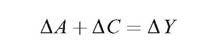
from which, by substituting in ΔC, we have

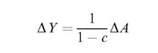
1/(1 — c) is the multiplier. If the propensity to consume is 0.8, an increase in the autonomous expenditure of $100 bn. will generate an increase in income of $500 bn. In fact, the initial expenditure of $100 bn. generates incomes that will be spent to buy consumer goods of the value of 0.8(100) = 80; this generates incomes which will be spent to buy consumer goods of the value of 0.8(80) = 0.64(100) = 64; and so on. Therefore, the overall income generated by the initial expenditure of 100 is equal to 100[1 + (0.8) + (0.8)² + (0.8)3 + (0.8)⁴ +... ] = 500. In fact, the sum of the numbers between the square brackets tends to 1/(1 — 0.8) = 5.

It is important to understand the reason why the multiplier process is convergent. A small increase in autonomous expenditure does not generate

unlimited growth of income. The reason for this is that there is a ‘leakage’ in the economic circuit. Every time there is an increase in income, part of it escapes from the expenditure circuit because it is saved. The ‘leakage’ in the simple multiplier is caused by savings. In more complex formulas, ‘leakages’ attributable to tax and imports are added. Signs of a rudimentary but deep insight into the multiplier process can be found in Marx. There is an inter­esting page in chapter 17 of the second volume of the Theories of Surplus Value, in which Marx tries to explain how a lack of effective demand in an industry with a high level of employment can be transmitted to the entire economy through a reduction in the production of that industry and the consequent reduction in employment and wages. The reduction in con­sumption which follows turns into a reduction in demand for other indus­tries, which, in turn, will be forced to reduce production and employment, generating a further reduction in effective demand. This process is linked to another deflationary process, consisting of a reduction in the demand for intermediate goods and for the means of production generated by the initial lack of demand and by the consequent reduction in the levels of activity which gradually spreads through the whole economy. The passage in which Marx explains this process is too brief and confused for us to be able to speak of a theory of the interaction between the multiplier and the accelerator, or even just a clear theory of the multiplier; but it is enough to show us that the problem had been posed long before it was solved.

About thirty years after Marx, there were some shrewd insights, if not something more, in an unpublished work of 1896 by Julius Wulff and in one by Nicolaus A. L. J. Johannsen, who used the ‘Multiplizirende Prinzip’, as he called it, to account for the effects produced by an initial impulse of expenditure on the whole economy.

However, the official date of birth of the multiplier is 1931. What hap­pened was that the theory, or rather a theory, of economic policy had shown the necessity for the multiplier principle. Keynes, expressing opinions cir­culating in Cambridge at those times, had raised the problem in Can Lloyd George Do It? (written in collaboration with H. Henderson in 1929), where he had put forward the argument that an increase in employment generated by public works would not be limited to the employment directly created by public expenditure but would generate additional induced employment. In the Treatise on Money of the following year, Keynes reproposed the argu­ment, but without managing to demonstrate it in a convincing way. How­ever, by now the time was almost ripe. In 1930 the multiplier principle was used by L. F. Giblin. Then in 1931 it was used by Jens Warming and by Ralph Hawtrey. Finally, the classic work of Richard Ferdinand Kahn, ‘The Relation of Home Investment to Unemployment’, came out in The Economic Journal of 1931. Keynes understood immediately that it was an important missing piece in the puzzle he was trying to solve, and in 1936 he assigned it a central place in the General Theory.

As to the accelerator, for the first traces we have to go back to a con­tribution by T. N. Carver of 1903. Then Albert Aftalion expressed it clearly in ‘La Realite des surproductions generales’ (1908-09). Finally it appeared in an article by C. F. Bickerdike and in one by John Maurice Clark.

In its simplest form the accelerator principle can be presented in the fol­lowing way. Let a be the marginal capital-output ratio, i.e. the increase in capital necessary to increase the production by a marginal amount. Then the expectation of an increase in the demand equal to ΔY* will induce entre­preneurs to make investments, I, in other words to increase the capital stock by an amount equal to: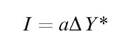

a is called the accelerator because, given that its value is normally greater than 1, the growth in capital is greater than the growth in the expected demand which induces it.

7.1.6. The Harrod-Domar Model

Right from the very beginning the accelerator was used to account for economic fluctuations. But the crucial year for the cycle theories based on the accelerator was 1936, when Roy Forbes Harrod published The Trade Cycle, in which he proposed an explanation of the business cycle which combined the accelerator and multiplier principles. Three years later Paul Anthony Samuelson put some order in this subject by combining the two principles with some special hypotheses on time lags and proving that it is possible to generate cyclical movements. But his demonstration was fatal for this line of research. In fact Samuelson proved that, generically, the cycles caused by the multiplier accelerator principle could be either dampened or explosive. Both properties are undesirable from the point of view of cycle theory, as they imply that the oscillating movements, in a certain sense, tend to extinguish themselves.

More promising was the line of research opened up by Harrod in ‘An Essay on Dynamic Theory’, published in the Economic Journal of 1939. Here the English economist, still using the multiplier-accelerator interaction, tackled the problem of the instability of growth. A few years later a similar theory was formulated by Evsey David Domar in various papers published in the 1940s and 1950s and later collected in Essays in the Theory of Economic Growth (1957). Thus the theory became known as the ‘Harrod-Domar model’.

In the simplest version it is based on three equations: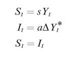

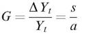
where s = 1 — c is the propensity to save, and Y* = Y* _{+ 1} — Y_t is the expected change in demand. The multiplier principle is hidden in the first equation, while the second incorporates the accelerator principle and the third sets out the condition of macroeconomic equilibrium. The equilibrium solution is obtained by substituting from the first and second equations into the third and assuming that the variation in the expected demand coincides with the actual one, i.e. DY* = Δ Y_t. The warranted rate of growth, G, which guar­antees equilibrium, is determined as:

The solution is unstable: each disequilibrium solution will tend to diverge from the warranted growth path, and no automatic adjustment mechanism is capable of rebalancing the economic system. For example, if the growth of expected demand is higher than warranted growth, the accelerator will increase investments more than necessary. The multiplier, in turn, will increase the demand at a rate higher not only than the warranted rate but also than the expected rate. Thus the expectations will be adjusted upwards and the disequilibrium will be aggravated.

Furthermore, given the growth rates of population and labour produc­tivity, the model shows that warranted growth, being unstable, is incapable of ensuring full employment and price stability. The sum of the rates of growth of population, n, and labour productivity, π, gives the natural rate of growth, G_n. This is the maximum rate at which the economy can grow. If demand grows at a rate higher than the natural one, this creates inflationary impulses, as actual production is not able to keep pace with demand. On the other hand, if demand grows at a rate lower than the natural one, unemploy­ment is created. The economy will grow in a steady state, without generating inflationary or deflationary impulses, if and only if it grows at a rate coinciding with both the warranted and the natural rates:

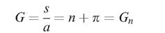
But as s, a, n, and π are all exogenous magnitudes, it is difficult to see how this equality can hold true, if not by chance.

In this section we have only sketched out the essential lines of the Harrod- Domar model. We will return to it in Chapter 9, where we deal with the theoretical developments to which it gave rise in the 1950s and 1960s. However, it is necessary to say something else about Harrod here.

The English economist believed that his most important scientific con­tribution was the Foundations of Inductive Logic (1956), a book which did receive serious consideration by eminent philosophers. In the field of eco­nomics, he believed that he was most competent in the analysis of the operation of the international monetary system; but he also made important

contributions to the theory of imperfect competition. Undoubtedly, however, his fame today is linked to the fact that he is the father of dynamic economics, with which he began to concern himself in 1939, even though his first work in this field dates back to 1934. As often happens with pioneering thinkers, Harrod was critical of the theoretical developments that others made from his original insights. This is true not only of the research linked to the neo­classical theory of economic growth but also, and more surprisingly, of the work connected to post-Keynesian theory. Both theories are, in fact, usually presented as extensions to the Harrod-Domar model. Yet Harrod has always refused to recognize his model as a realistic description of the actual dynamics of a capitalist economy, a dynamic which is considered as basically characterized by continual cyclical fluctuations. Undoubtedly, the almost uninterrupted growth of the Western economies from the end of the Second World War to the 1970s has contributed to legitimating the steady growth models and left Harrod’s original views in the shadows. However, the period of deep instability we are now passing through favours a general reappraisal of the economic-growth argument which may lead to a re-examination and a new appreciation of the Keynesian bases of post-Keynesian theory. From this perspective, Harrod’s original work takes on new interest.

7.2.