Consumption and Labor Supply in a Two-Period Competitive Model

We next turn to an intertemporal, two-period model of consumption and labor supply. For reasons of analytical simplicity, as in the model of section 2.4, we abstract from capital accumulation.

Thus, the representative household chooses consumption and employment in both periods, given its endowments of time in periods 1 and 2, a competitive real interest rate for its savings, and competitive real wages in periods 1 and 2.

2.5.1 Optimal Consumption and Labor Supply in a Two-Period Model

Assume a representative household that lives for two periods, 1 and 2. Also assume that the representative household is endowed with one unit of labor for each of periods 1 and 2. In both periods, its endowment of time can either be used as leisure (which yields utility to the household) or rented as labor to private firms at competitive real wages w₁ and w₂. Labor is used by competitive firms in the production of a single good in both periods y₁ and y₂.

The household can use its labor income for consumption in each period. Savings from period 1 to 2 can be lent in competitive financial markets at a competitive real interest rate r. Obviously, there are no savings in period 2. There is also no uncertainty, and the household has perfect foresight.

The representative household is assumed to maximize the intertemporal utility function

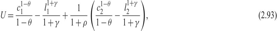
subject to the intertemporal budget constraint

The first-order conditions for the maximum are

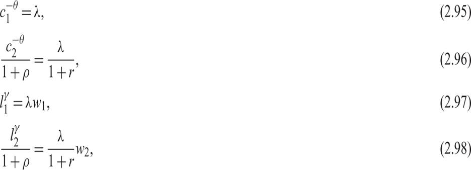
where λ is the Lagrange multiplier of the constraint (2.94).

The economic interpretation of these first-order conditions is straightforward. (2.95) implies that the marginal utility of first-period consumption is equal to the marginal value of wealth. (2.96) implies that the marginal utility of second-period consumption is equal to the discounted marginal value of wealth. (2.97) implies that the marginal utility of first-period leisure is equal to the opportunity cost of leisure (i.e., the real wage in period 1 multiplied by the marginal value of wealth). Finally, (2.98) implies that the marginal utility of second-period leisure is equal to the opportunity cost of leisure (i.e., the real wage in period 2 multiplied by the discounted marginal value of wealth). The discount factor is inversely related to the real interest rate r.

2.5.2 Intertemporal Substitution in Consumption and Labor Supply

Eliminating λ between (2.95) and (2.96) gives us the Euler equation for consumption:

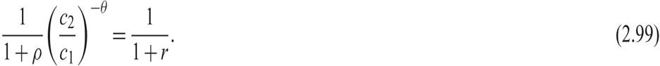
This is the same as the Euler equation for consumption (2.41) in the model with exogenous labor supply and has the same interpretation. At the optimum, the marginal rate of substitution between future and current consumption is equal to the marginal rate of transformation of future consumption into current consumption (or the opportunity cost [price] of future consumption). This rate is equal to the inverse of one plus the real interest rate r.

Eliminating λ between (2.97) and (2.98) gives us a corresponding Euler equation for labor supply:

This is a new optimality condition relative to the two-period model with exogenous labor supply. At the optimum, the marginal rate of substitution between future and current leisure (employment) is equal to the marginal rate of transformation of future leisure into current leisure (or the opportunity cost [price] of future leisure).

(2.100) suggests that the household will not only engage in intertemporal substitution in consumption, as suggested by (2.99), but also in intertemporal substitution in labor supply. When discounted future wages are higher than current wages, the household will reduce its current labor supply in favor of future labor supply, and vice versa.

The importance of (2.100) is that fluctuations of employment over time will not only depend on fluctuations in real wages but also on fluctuations in the real interest rate.¹¹

Eliminating λ between (2.95) and (2.97), and (2.96) and (2.98), respectively, gives us the optimality conditions for the choice between consumption and leisure in each period (i.e., the marginal rate of substitution between consumption and leisure must be equal to the real wage in both periods):

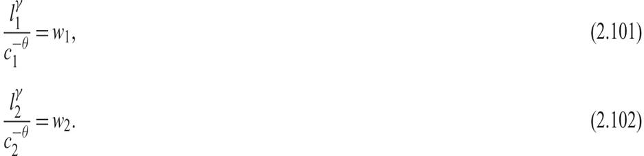
These are the same conditions as in the static model of section 2.3.

This completes our examination of the optimal decisions of the representative household.

2.5.3 Optimal Production Decisions of Firms

Assume that output is produced by competitive firms and that labor is the only factor of production. The production functions of firms are given by

where A > 0 is total factor productivity in period 1, and g ≥ 0 is the growth rate of total factor productivity between periods 1 and 2. Here, g is an exogenous parameter measuring technical progress. This is the same technology as assumed in the one-period model with endogenous labor supply, the only difference being that total factor productivity is allowed to grow between periods.

Firms are assumed to maximize profits. Hence, in each period, they choose labor to maximize

From the first-order conditions for a maximum, we have

Because firms operate in competitive markets, they all face the same real wage.

Note that, because of the assumption of constant returns to scale, wage payments to households exhaust output. Firms pay to households the real wage bill wl in each period. The real wage w is equal to total factor productivity, so that

The income of the representative household is equal to aggregate output in each of the two periods.

2.5.4 General Equilibrium and the Determination of Output and Employment

To determine the employment rates in each period (and through the employment rates, the rest of the endogenous variables), we must consider the equilibrium conditions in product, labor, and financial markets. Hence we must combine the optimal decisions of firms with the optimal decisions of households. This will allow us to determine all the endogenous variables.

Because there is no capital (i.e., an outside asset for savings), households that wish to save in period 1 can only lend to households that wish to borrow in period 1. However, because all households have the same endowments and preferences, and they face the same real wages and real interest rate, all households will wish to be either a net lender or a net borrower at any given interest rate. As there cannot be an equilibrium with either positive or negative savings, the interest rate adjusts to ensure that the representative household consumes all its current income in every period, and there are no savings. This is the equilibrium condition in financial and product markets, which determines the real interest rate. If there were an outside asset, like capital, then the equilibrium condition would have been that savings are equal to investment.

Using the definition of household income (2.106) and the budget constraint of the representative household (2.75), we get that consumption in every period is also a function of the employment rate:

These are the equilibrium conditions in the product market, ensuring that the consumption decisions of households are compatible with the production decisions of firms.

Equilibrium employment makes the employment decisions of households (as given by (2.101) and (2.102)) equal to the employment decisions of firms (as given by (2.105)). As a result, we have

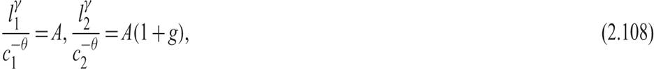
which is the set of equilibrium conditions in the labor market, ensuring that the real wage w is compatible with the employment decisions of both households and firms in every period.

Solving (2.107) and (2.108) simultaneously, we can determine the equilibrium employment rates. The solutions for the equilibrium l₁ and l₂ are given by

where l denotes equilibrium employment. From (2.109), equilibrium employment will be a positive function of productivity A and productivity growth g only if θ < 1 (i.e., only if 1/θ, the intertemporal elasticity of substitution of consumption, is greater than unity).

If the intertemporal elasticity of substitution of consumption is greater than unity, then the period with higher productivity will be the period with higher employment as well, as households will wish to work more and so have higher income and consumption. The intertemporal substitution effect is stronger than the income effect in this case. The opposite happens if the intertemporal elasticity of substitution of consumption is less than unity.

Note that if the intertemporal elasticity of substitution of consumption is equal to unity or if the Frisch elasticity of labor supply is equal to zero, then equilibrium employment is constant and equal to unity and does not depend on productivity or productivity growth.

Because there is no outside asset as an outlet for savings, the equilibrium real interest rate adjusts to ensure that consumption is equal to income in both periods.

This equation defines the equilibrium real interest rate that ensures that the intertemporal decisions of the representative household are consistent, in the sense that savings are equal to investment. Because there is no capital in this model and investment is equal to zero, the equilibrium real interest rate ensures that savings are equal to zero.

The equilibrium real interest rate is a positive function of the pure rate of time preference and also of the rate of growth of productivity. Thus, both the preferences of the representative household and the technology of production affect the equilibrium real interest rate.

For a given rate of growth of productivity, the real interest rate increases with increasing θ (i.e., it decreases with decreasing intertemporal elasticity of substitution of consumption 1/θ). The more difficult it is for households to substitute consumption intertemporally, the higher the equilibrium real interest rate will be.

By taking the logarithm of the real interest rate, the equilibrium condition (2.110) can be approximated by

If the intertemporal elasticity of substitution of consumption 1/θ is equal to unity, then the equilibrium real interest rate is equal to ρ + g, the sum of the pure rate of time preference and the growth rate of productivity.

Equilibrium real wages and equilibrium output and consumption are determined by

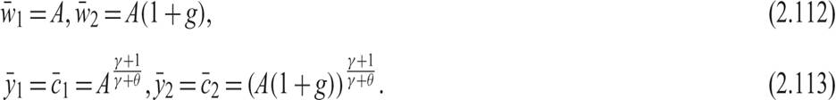
The equilibrium real wage is equal to the exogenous total factor productivity, which for a linear production function is equal to the marginal productivity of labor. Thus, real wages grow at a rate g between periods 1 and 2.

Equilibrium output and consumption are also positive functions of total factor productivity. If the intertemporal elasticity of substitution of consumption is higher than unity (i.e., θ < 1), then the elasticity of equilibrium aggregate output and consumption with respect to total factor productivity is greater than unity as well, as higher productivity induces higher employment from households, and vice versa.

Exercise 2.4 Assume that the representative household is endowed with l₀ units of labor in each period and lives for two periods. There is no capital. Derive equilibirum production, consumption, the real interest rate, and the real wage for each period, assuming that households maximize utility subject to the relevant resource constraints, firms maximize profits, and product and factor markets are competitive. Assume a CEIS intertemporal utility function of the form (2.93) and production functions of the form (2.103). Discuss how the equilibrium depends on the labor endowment, preferences, and technological parameters. How are your conclusions modified if the elasticity of intertemporal substitution of consumption is equal to unity?

2.5.5 Implications for Business Cycle Theory

The two-period model of consumption and labor supply that we have examined in this section is the basis of most dynamic stochastic general equilibrium (DSGE) models of aggregate fluctuations.

The stochastic growth model analyzed in chapter 13 (which is the basis of most real business cycle models) and the new classical model of aggregate fluctuations without capital (analyzed in chapter 14) are direct extensions of the two-period model of consumption and labor supply to economies that last for an infinite number of periods. These models are subject to random disturbances to total factor productivity. However, much like the two-period model of this section, these models assume full and perfectly competitive markets, and the absence of market distortions, such as wage and price rigidity. As we shall see in chapters 13 and 14, the optimality conditions of the two-period model, such as the Euler equation for consumption and the individual optimality conditions for labor supply, recur again and again in these infinite-horizon competitive models. Hence, the key properties of these infinite-horizon competitive models are quite closely related to the two-period model.

New Keynesian models of aggregate fluctuations are extensions of the two-period model to monetary economies that are characterized by both real and nominal distortions and disturbances in product and labor markets. Such new Keynesian models relax the assumptions of full and competitive markets, as well as the assumption of perfect wage and price flexibility. They imply that the resulting macroeconomic equilibria are suboptimal. Such models are analyzed in chapters 16 and 17.

A more recent development is the extension of new Keynesian models to models including financial distortions as well. This was a direct result of the financial crisis of 2008–2009. Models of fully efficient financial markets are gradually giving way to models of financial frictions and the absence of perfect capital markets. Such models are introduced and discussed in chapter 19 on financial frictions.

2.6