A Perfectly Competitive Model without Capital
In what follows, we focus on a perfectly competitive new classical model of aggregate fluctuations, in which the only variable factor of production is labor. For analytical simplicity, we thus abstract from capital accumulation, which is an important propagation mechanism in the stochastic growth model that we analyzed in chapter 13.
In this analytically simpler model, we allow for a more general approach to the preferences of the representative household and also distinguish between nominal and real variables. This allows us to consider the determination of the level of prices and wages, inflation and nominal interest rates, and the role of monetary factors in new classical models.
14.1.1 The Representative Household
The representative household is assumed to maximize

where C is consumption, and L is labor supply. We assume that

The constraints under which the maximization takes place are given by
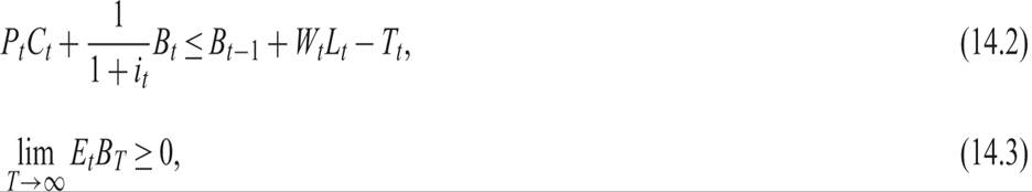
where P is the price level, W is the nominal wage, i is the nominal interest rate, B is a nominal one-period bond, and T is the level of exogenous nominal taxes minus exogenous transfers of nominal income to the household.
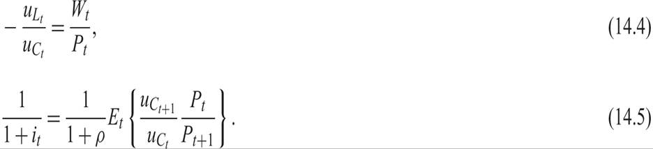
From the first-order conditions, it follows that
Assume that the per period utility function is given by

where θ > 0, λ > 0, 1/θ is the intertemporal elasticity of substitution in consumption, and 1/λ the Frisch elasticity of labor supply.2
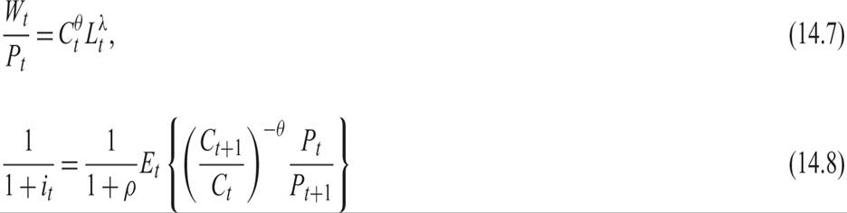
The first-order conditions for the problem of the representative household in this case take the form
Equations (14.7) and (14.8) can be written in log-linear form as
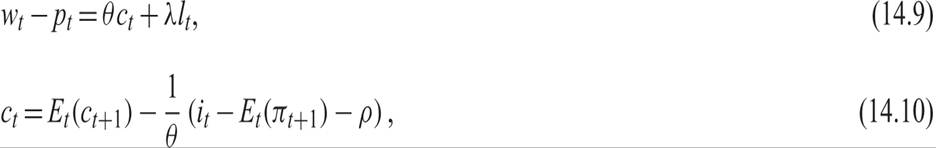
where w = ln W, p = ln P, c = ln C, l = ln L, and πt = pt − pt−1 is the inflation rate.
14.1.2 The Representative Firm
Production of the representative firm is a positive function of employment and is described by an aggregate production function of the form

where A > 0 and 0 < α < 1 are exogenous technological parameters; α is a constant, and A follows an exogenous stochastic process.
The representative firm chooses employment to maximize profits, for given nominal wages and prices. Profits are determined by

Profit maximization implies that employment will be determined so as to equate the marginal product of labor to the real wage:

One can solve the marginal productivity condition for employment. The interpretation is that labor demand is a negative function of the deviation of real wages from productivity:
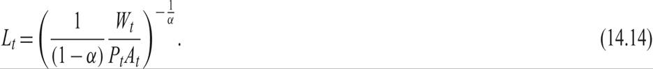
One can also solve the marginal productivity condition for the price level. The interpretation is that the product price is equal to marginal cost:

Log-linearizing the first-order condition (14.13), we get

where a = lnA. Log-linearizing the production function (14.11), we get

Having determined the behavior of households and firms, we can now analyze general equilibrium in this model.
14.1.3 General Equilibrium
Because we have assumed that there is no investment or public consumption, in product market equilibrium, consumption will be equal to total output:

The equilibrium condition (14.18) will determine the real interest rate.
The condition for equilibrium in the labor market will require that labor demand, as implied by (14.16), should be equal to labor supply, as implied by (14.9). This will determine the real wage.
The model consists of equations (14.9), (14.10), (14.16), (14.17), and the equilibrium condition (14.18). It determines employment, output, consumption, real wages, and the real interest rate as functions of the exogenous labor productivity process a.
The real interest rate is defined by the Fisher equation as

Solving the model for the five endogenous variables, we get

where 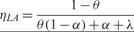 and
and 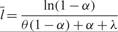 ;
;

where 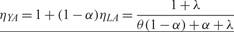 , and
, and  ;
;

where 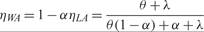 , and
, and 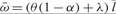 ; and
; and

Equations (14.20)–(14.23), along with the product market equilibrium condition (14.18), determine the five endogenous variables as log-linear functions of the exogenous labor productivity process a.
Note that fluctuations in employment, output, consumption, and real wages are functions only of fluctuations in exogenous labor productivity at, and fluctuations in the real interest rate depend on fluctuations in the expected rate of change of productivity at.
Output, consumption, and real wages are positive functions of productivity, whereas employment is a positive function of productivity only if θ < 1 (i.e., if the intertemporal elasticity of substitution of consumption is greater than one). If θ > 1, employment is a negative function of productivity; but if θ = 1, employment is independent of productivity. This is because if θ < 1, the substitution effect dominates over the income effect, after a change in productivity, and real wages, and employment rise. If θ > 1, the income effect dominates over the substitution effect. In the case θ = 1, the two effects cancel each other out, and employment is not affected by the productivity shock.
Only real factors (such as real productivity) affect fluctuations in real variables. As in the stochastic growth model, monetary factors (such as the money supply and nominal interest rates) have no impact on the evolution of real variables.
14.2
More on the topic A Perfectly Competitive Model without Capital:
- Alogoskoufis George. Dynamic Macroeconomics. The MIT Press,2019. — 800 p., 2019
- Capital-Skill Complementarity in an Overlapping Generations Model
- The Value of One’s Contribution
- Limitations of the Market
- Hicks’s Non-welfarist Manifesto: Its Depth and Reach
- GREEN UNPLEASANT LAND
- XAT 2009